Dynamic Programming for 0/1 Knapsack

1. Understanding the 0/1 Knapsack Problem

Imagine you're a burglar with a knapsack. You've entered a house with several items, each with a specific weight and value. Your knapsack has a maximum weight capacity. Your goal is to choose which items to steal to maximize the total value of your haul, without the total weight of the items exceeding your knapsack's capacity.

The "0/1" part of the name means that for each item, you have a binary choice: you either take the entire item (1) or you leave it behind (0). You cannot take a fraction of an item.

Let's formalize this:

• You have $n$ items.
• Each item $i$ has a weight $w_i$ and a value $v_i$.
• Your knapsack has a maximum weight capacity of $W$.
• You want to choose a subset of items that maximizes $\sum v_i$ subject to $\sum w_i\le W$.

Why Not a Greedy Approach?

Your first instinct might be to use a greedy strategy. For example:

1. Take the most valuable items first.
2. Take the lightest items first.
3. Take the items with the highest value-to-weight ratio ($v_i/w_i$) first.

While these sound plausible, they don't guarantee an optimal solution. A single, high-value item might take up all the space, preventing you from picking several other items that, combined, would have been more valuable.

Since greedy approaches fail, we need a method that explores all possibilities in a structured way to find the true optimum. This is where Dynamic Programming excels.

2. Formulating the DP Solution

As we've learned, the key to DP is to break the problem down into smaller, overlapping subproblems.

The Recursive Structure

Let's define our subproblem: "What is the maximum value we can obtain considering only the first i items with a knapsack capacity of w?"

Let's create a function, knapsack(i, w). When considering the $i$-th item, we have two choices:

1. Don't take the item: If we don't take item $i$, the problem reduces to finding the maximum value we can get from the first $i-1$ items with the same capacity $w$. The value is simply knapsack(i-1, w).
2. Take the item: We can only do this if the item's weight, $w_i$, is less than or equal to the remaining capacity, $w$. If we take it, we gain its value, $v_i$, but our remaining capacity decreases by $w_i$. The problem then reduces to finding the maximum value from the first $i-1$ items with a capacity of $w-w_i$. The value is v_i + knapsack(i-1, w - w_i).

Since we want to maximize the value, we take the best of these two choices. This gives us our recurrence relation:

The base cases for the recursion are:

• If we have no items left ($i=0$) or no capacity left ($w=0$), the maximum value is 0.

This recursive approach has exponential time complexity due to re-calculating the same subproblems repeatedly. We can optimize this using memoization (top-down) or tabulation (bottom-up). Let's focus on the tabulation method, as it's often more intuitive for visualizing the DP solution.

The Tabulation (Bottom-Up) Approach

We can solve this problem iteratively by building a 2D table (or matrix). Let dp[i][w] be the maximum value achievable using items from 1 to $i$ with a total capacity of $w$.

• The rows of our table will correspond to the items (from 0 to $n$).
• The columns will correspond to the knapsack capacity (from 0 to $W$).

The final answer to our problem will be the value in the bottom-right cell, dp[n][W].

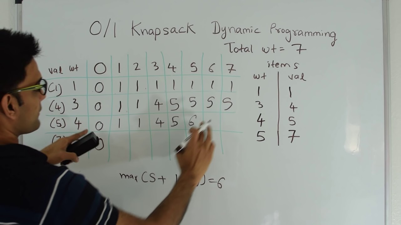
We fill the table row by row, item by item. For each cell dp[i][w], we apply our recurrence relation:

dp[i][w] = max(dp[i-1][w], v[i-1] + dp[i-1][w - w[i-1]])

• dp[i-1][w] corresponds to the "don't take item $i$" case.
• v[i-1] + dp[i-1][w - w[i-1]] corresponds to the "take item $i$" case. (Note the i-1 index for v and w arrays if they are 0-indexed).

3. Reconstructing the Solution

The DP table gives us the maximum value, but what if we need to know which items were selected to achieve this value? We can find this by tracing our steps backward from the final cell dp[n][W].

Here's the logic:

1. Start at dp[i][w] where i=n and w=W.
2. Compare dp[i][w] with dp[i-1][w].
   • If they are equal (dp[i][w] == dp[i-1][w]), it means item $i$ was not included in the optimal solution for this subproblem. So, we move up to dp[i-1][w].
   • If they are not equal, it means item $i$ was included. We add item $i$ to our list of chosen items. Its inclusion contributed v[i-1] to the value, so we must have come from the subproblem before this item was added. We move diagonally up and to the left, to dp[i-1][w - w[i-1]].
3. Repeat this process until we reach the first row ($i=0$).

4. Complexity Analysis and Optimization

Let's analyze our tabulation solution.

• Time Complexity: We are filling a 2D table of size $(n+1)\times (W+1)$. Each cell takes constant time to compute. Therefore, the time complexity is $O(n\cdot W)$.
• Space Complexity: We store the entire 2D table, so the space complexity is also $O(n\cdot W)$.

This is known as a pseudo-polynomial time complexity. The runtime depends on the numeric value of the input W, not just the number of items n. If W is very large, this can be slow, but for typical constraints, it's very effective.

Space Optimization

This is a perfect moment to apply what we learned in the last lesson. Look at the recurrence relation again:
dp[i][w] = max(dp[i-1][w], ... + dp[i-1][...])

Notice that to compute the values for the current row i, we only ever need values from the previous row i-1. We never need to look at i-2, i-3, etc. This is the exact condition for applying the rolling array optimization!

We can reduce the space complexity from $O(n\cdot W)$ to $O(W)$ by only keeping track of the previous row and the current row.

Even better, for the 0/1 Knapsack problem, we can optimize it down to a single 1D array of size $O(W)$. The trick is to iterate through the capacities w in reverse order (from W down to w_i). This ensures that when we compute dp[w], we are using the values from the previous item's iteration for dp[w - w_i], not the values we've just updated for the current item.

Here's the space-optimized Python code from the article for your reference:

def knapsack_optimized(W, val, wt):
    n = len(wt)






    # We only need a 1D array for DP
    dp = [0] * (W + 1)







    # Iterate through each item
    for i in range(n):






        # Iterate backwards through capacities
        for w in range(W, wt[i] - 1, -1):






            # Apply the recurrence
            dp[w] = max(dp[w], val[i] + dp[w - wt[i]])
    
    return dp[W]

Note that with this optimization, we lose the ability to easily backtrack and find the chosen items, as we no longer store the full table.

Conclusion

Congratulations on mastering your first classic DP problem! The 0/1 Knapsack is a cornerstone of algorithm studies because it beautifully demonstrates the power of DP to solve problems that are intractable with naive or greedy methods.

Key Takeaways:

• The 0/1 Knapsack problem seeks to maximize value within a weight constraint.
• Greedy strategies fail because local optimal choices do not guarantee a global optimum.
• The DP solution relies on a recurrence relation with two choices for each item: take it or don't take it.
• A bottom-up (tabulation) approach builds a 2D table dp[i][w] to find the optimal value. The time and space complexity are both $O(n\cdot W)$.
• The set of chosen items can be found by backtracking through the filled DP table.
• The space complexity can be optimized from $O(n\cdot W)$ to $O(W)$ by observing that each row only depends on the previous one.

Preview of the Next Lesson:
We will continue our journey through classic DP problems by tackling the Longest Common Subsequence (LCS) problem. This problem has a slightly different structure and is fundamental to many real-world applications, such as diff utilities (comparing file changes) and bioinformatics (analyzing DNA sequences).