Solving the Coin Change Problem

1. Understanding the Coin Change Problem

The problem statement is as follows:

Given a set of coin denominations (e.g., {1, 5, 10, 25}) and a target amount A, find the minimum number of coins that sum up to A. You can assume an unlimited supply of each coin denomination.

For example, to make change for $20 with coins {$5, $10, $20}, you could use four $5 coins, two $10 coins, or one $20 coin. The optimal solution is one coin.

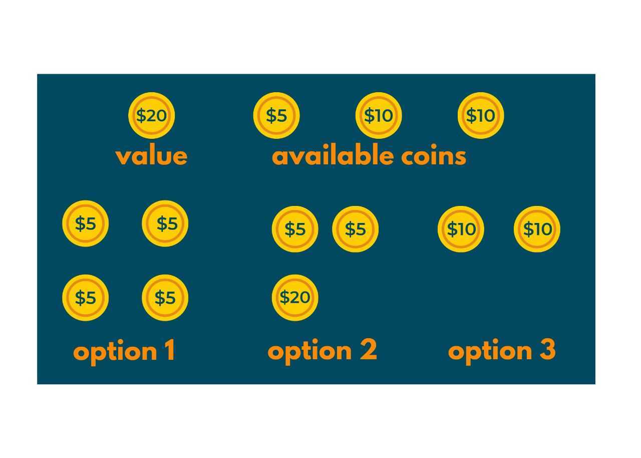
If it's impossible to make the target amount, we typically return an indicator like -1 or infinity.

2. Formulating the DP Solution

Like other DP problems, Coin Change has the properties of optimal substructure and overlapping subproblems.

• Optimal Substructure: The minimum number of coins to make amount A can be found by first using one coin (say, of value c) and then finding the minimum number of coins for the remaining amount A - c. The optimal solution for A is built upon the optimal solutions for smaller amounts.
• Overlapping Subproblems: When calculating the solution for A, you might find yourself recalculating the solution for a smaller amount (e.g., A - 5 - 1 and A - 1 - 5) multiple times.

This structure suggests that we can define our subproblem as:
Let dp[i] be the minimum number of coins required to make change for amount i.

Our goal is to compute dp[A].

Top-Down Intuition (Recursion)

A natural way to think about this is recursively. To find the minimum coins for an amount A, we can try using each available coin c as the last coin. If we use coin c, the total number of coins will be 1 + (minimum coins for amount A - c). We do this for all possible coins and take the minimum.

This recursive approach, however, leads to many redundant calculations. The video below does an excellent job of visualizing this recursion as a tree and highlighting the duplicate subproblems that make it a perfect candidate for dynamic programming.

3. The Bottom-Up (Tabulation) Approach

While the top-down approach is intuitive, the bottom-up approach is often more efficient to implement iteratively. We'll build a 1D array, dp, of size A + 1, where dp[i] will store the minimum coins for amount i.

1. Initialization:

   • dp[0] = 0, because zero coins are needed to make an amount of 0.
   • Initialize all other dp[i] to a large value (like infinity or A + 1) to signify that they are not yet reachable. An amount A can never require more than A coins (if a 1-cent coin exists), so A+1 serves as a good stand-in for infinity.

2. Iteration: We iterate from i = 1 up to A. For each amount i, we iterate through our available coin denominations c. If a coin c is less than or equal to i, we can potentially use it. The recurrence relation is:

   $$dp[i]=\min (dp[i],1+dp[i-c])$$

   In words: the minimum coins for amount i is the minimum of its current value and 1 + (the minimum coins for amount i - c). We update dp[i] for each coin we can use.

This process systematically builds the solution from amount 1 all the way to A, ensuring that when we calculate dp[i], the values for all smaller amounts (like dp[i-c]) have already been optimally computed.

The following video provides a step-by-step walkthrough of filling this DP table. Seeing it done visually is often the best way to solidify the concept.

A More Formal View

For a more formal, mathematical perspective, we can reference the tutorial solutions from the University of Toronto. While they initially define a 2D array, they also describe the more common 1D array approach we've just discussed.

The recurrence D[i] = 1 + min_{j:d[j]≤i} D[i −d[j]] is precisely the logic we apply in our nested loops: for a given amount i, we find the minimum over all possible coin choices j.

4. Complexity Analysis

Your preference for understanding the "why" includes analyzing performance. Let's break down the complexity of our bottom-up solution.

• Time Complexity: $O(A\times C)$

  • We have an outer loop that runs from 1 to A (the target amount).
  • Inside it, we have an inner loop that iterates through all C coin denominations.
  • This gives us a total time complexity proportional to the amount multiplied by the number of coins.

• Space Complexity: $O(A)$

  • We need an array of size A + 1 to store the intermediate solutions for each amount from 0 to A.

The presenter in the video LINK confirms this analysis in the final part of the video (20:05 - 22:12).

5. A Note on Variations

The "Coin Change" problem is a family of problems. The version we solved is the most common one, sometimes called Unbounded Knapsack because you have an unlimited supply of each item (coin).

It's useful to be aware of two other major variations:

1. Total Unique Ways to Make Change (Coin Change 2): Here, the goal is not to find the minimum number of coins, but to count the number of distinct combinations of coins that sum to the target amount. This requires a different DP state and recurrence. The video "Total Unique Ways To Make Change" (LINK) covers this variant if you're curious.

2. Minimum Coins with Limited Supplies (Bounded Knapsack): This is the version where you have a finite count of each coin denomination (e.g., three 5-cent coins, two 10-cent coins). This adds another dimension to the problem, making it more similar to the 0/1 Knapsack problem we've already seen. The article "Tackling the 'Minimum Coins with Limited Supplies' Problem" (LINK) explores this more complex scenario.

Being able to distinguish between these variants is a key skill in applying the correct DP pattern.

Conclusion

In this lesson, we mastered the classic Minimum Coin Change problem using dynamic programming. This concludes our module on foundational DP applications.

Key Takeaways:

• The Minimum Coin Change problem seeks the fewest coins to form a target amount, assuming an unlimited supply of each denomination.
• The optimal subproblem is defined as dp[i]: the minimum coins needed to make change for amount i.
• The recurrence relation for the bottom-up approach is dp[i] = min(dp[i], 1 + dp[i - c]) for each coin c.
• The solution has a time complexity of $O(Amount\times |Coins|)$ and a space complexity of $O(Amount)$.

Preview of the Next Lesson:
We are now ready to move into our next module, "Advanced Algorithmic Patterns". We'll begin by looking at algorithms on graphs, specifically Topological Sorting on a Directed Acyclic Graph (DAG). This is a fundamental operation with applications in scheduling tasks, resolving dependencies in software builds, and more.