Hello! Welcome to the next lesson in our exploration of Dynamic Programming.
In the previous lesson, we transformed an inefficient, purely recursive Fibonacci function into a linear-time solution using memoization. We established that this is a top-down approach: we start with our goal and use recursion to solve smaller subproblems, caching the results along the way to avoid re-computation.
Today, we'll learn the other fundamental DP implementation strategy: tabulation. Your learning outcome is to convert a top-down memoized solution to a bottom-up tabulation approach. This will give you a complete picture of the two main ways to code a DP solution.
1. From Top-Down to Bottom-Up: Introducing Tabulation
While memoization starts from the top and works down, tabulation does the exact opposite. It's a bottom-up approach.
The core idea is to solve the problem iteratively, starting with the smallest, simplest subproblems (the base cases) and building up towards the final solution. We use a table (typically an array, hence "tabulation") to store the results of these subproblems.
Think of it this way:
- Memoization (Top-Down) is like a manager asking for a final report. The manager asks a subordinate for a key figure, who in turn asks another, and so on, down to the base data. When a figure is calculated, it's jotted down so no one has to calculate it again.
- Tabulation (Bottom-Up) is like an analyst starting with the raw data. The analyst first calculates all the basic figures, puts them in a spreadsheet, then uses those to calculate intermediate figures, and continues row by row until the final report figure is computed.
This image provides a great visual summary of the two concepts:
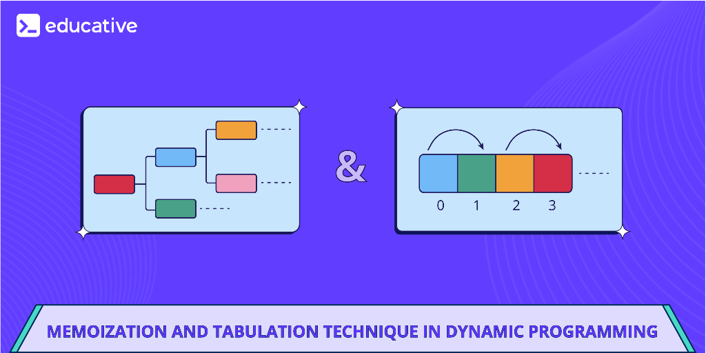
Let's see this in action with our familiar Fibonacci example.
4 Principle of Optimality - Dynamic Programming introduction
The Abdul Bari video we watched in the last lesson also provides an excellent introduction to tabulation, directly contrasting it with the memoization approach we just learned.
Watch the segment from 11:42 to 14:36. Observe how an iterative loop is used to fill an array starting from the base cases F(0) and F(1), building up to the final answer.
As the video shows, for Fibonacci, we can create an array dp of size n+1. We initialize dp[0] = 0 and dp[1] = 1. Then, we loop from i = 2 to n, calculating each dp[i] using the values we've already stored: dp[i] = dp[i-1] + dp[i-2].
2. The Conversion Process: A Systematic Approach
Converting a recursive, memoized solution into an iterative, tabulated one is a key skill. It's a structured process that can be broken down into a few steps. Since your background is in engineering and software development, you'll likely appreciate this methodical approach.
The general process is:
- Define the DP Table: Determine the dimensions and size of your table. This is guided by the state variables in your memoized solution (i.e., the parameters of the recursive function). For
fib(n), the state is justn, so we need a 1D array. For a function likesolve(i, j), you'd need a 2D table. - Initialize Base Cases: Fill in the table entries that correspond to the base cases of the recursion. For Fibonacci, this means setting
dp[0]anddp[1]. - Determine Iteration Order: This is the most critical step. You must design your loops to iterate through the subproblems in an order that guarantees a subproblem's solution is calculated before it is needed by another. In the Fibonacci recurrence ,
F(n)depends on smaller indices, so our loop must go from smallnto largen. - Translate the Recurrence: The body of your loop will implement the recurrence relation, but instead of making recursive calls, it will perform lookups in your DP table.
fib(i-1)becomesdp[i-1].
The following video provides an excellent, in-depth guide to this conversion process using a more complex example (the Coin Change problem). While the problem itself is more advanced, the principles for conversion are universal and clearly explained.
Recursive to iterative dynamic programming in 3 steps!
The video 'Recursive to iterative dynamic programming in 3 steps!' from the channel DecodingIntuition offers a robust framework for this conversion.
Watch the following three segments, focusing on the process, not just the specific problem: Figuring out the Table (1:20 - 5:00): This covers Step 1, identifying the function parameters to define the DP array dimensions. Figuring out the Loop Order (5:00 - 8:40): This is the core logic for Step 3, analyzing dependencies in the recurrence to determine the correct loop order. Replacing Recursion with Array Access (10:42 - 12:31): This covers Step 4, showing the direct translation of recursive calls to table lookups.
The key insight from the video is that the structure of the recurrence relation dictates the structure of your loops. By analyzing which subproblems f(i, j) depends on, you can deduce whether your loops for i and j should be increasing or decreasing.
3. Memoization vs. Tabulation: Key Differences
Now that you've seen both approaches, let's formally compare them. Both have the same goal—avoiding redundant work—but they have different characteristics and trade-offs.
The GeeksforGeeks article 'Tabulation vs Memoization' provides a concise summary and a clear comparison table.
First, read the brief introduction to remind yourself of the high-level definitions. Then, carefully study the comparison table under the 'Tabulation vs Memoization' heading. It contrasts the two techniques on several important axes.
Here is a summary of the most important points from that table:
| Aspect | Memoization (Top-Down) | Tabulation (Bottom-Up) |
|---|---|---|
| Approach | Recursive. Starts from the final state and breaks it down. | Iterative. Starts from the base states and builds up. |
| Execution | Slower due to recursion overhead (function calls, stack management). | Faster due to direct iteration and no recursion overhead. |
| State Space | Only solves subproblems that are actually required to reach the final state. | Solves all subproblems up to the final state, which might include some unnecessary ones. |
| Code | Often more intuitive to write, as it closely follows the pure recursive logic. | Can sometimes be harder to reason about the correct loop order and initialization. |
For many problems, like Fibonacci, where all subproblems up to n are needed anyway, tabulation is often preferred for its slightly better performance by avoiding recursion overhead. However, if the state space is sparse and only a fraction of subproblems need to be solved, memoization can be more efficient by not computing unused states.
To see the conversion in practice on another problem, you can skim the "Rod Cutting Problem" sections in the same GeeksforGeeks article (LINK). Compare the memoized solution (Section: Using Top-Down DP) with the tabulated one (Section: Using Bottom-Up DP). You'll notice the same pattern: the recursive calls in the first are replaced by array lookups and loops in the second.
Conclusion
Today, you've learned about tabulation, the second pillar of dynamic programming implementation. By understanding both memoization and tabulation, you now have two powerful tools to choose from when solving DP problems.
Key Takeaways:
- Tabulation is a bottom-up, iterative approach to dynamic programming.
- It works by filling a table with solutions to subproblems, starting from the base cases and building up.
- Converting a memoized solution to a tabulated one involves defining a table, initializing base cases, determining the correct loop order based on dependencies, and translating the recurrence into iterative table lookups.
- Tabulation avoids recursion overhead and is often slightly faster, while memoization can be more intuitive to write and may be better for problems with sparse subproblem spaces.
Preview of the Next Lesson:
We've successfully converted a solution from recursive to iterative. In the next lesson, we'll formalize the analysis of time and space complexity for dynamic programming solutions. We'll also explore a common and powerful follow-up step: space optimization, where we can often reduce the memory footprint of our tabulated solutions significantly. For instance, the Fibonacci problem can be solved with space instead of .