Hello! Welcome to your next lesson.
In our last session, we mastered Kruskal's algorithm, an "edge-centric" greedy method that finds a Minimum Spanning Tree (MST) by sorting all edges and adding the cheapest ones that don't form a cycle. We saw how the Union-Find data structure was the perfect tool for that job.
Today, we will explore another classic algorithm for the same problem: Prim's algorithm. Prim's also uses a greedy strategy, but it takes a "vertex-centric" approach. Instead of building a forest of trees like Kruskal's, it grows a single tree from a starting point, one vertex at a time. Your goal for this lesson is to learn how to apply Prim's algorithm using a priority queue to find an MST.
1. The Core Idea: Growing a Single Tree
Prim's algorithm works by partitioning the graph's vertices into two sets:
- Vertices already included in the MST.
- Vertices not yet included.
The algorithm starts with an arbitrary vertex in the first set. Then, at each step, it greedily selects the edge with the minimum weight that connects a vertex from the first set to a vertex in the second set. This new vertex and edge are then added to the MST. This process continues until all vertices are in the MST.
Because it always picks the cheapest edge to expand the tree, the algorithm feels like it's organically growing outward from the starting node.
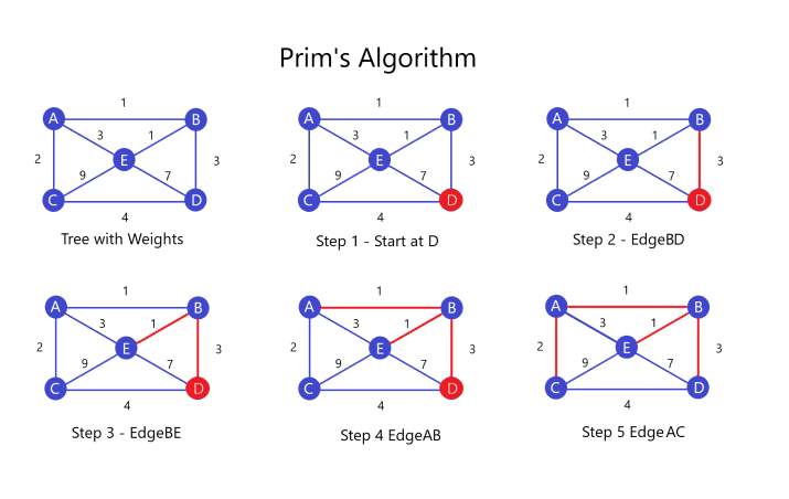
This vertex-centric growth is the key difference from Kruskal's algorithm, which considers edges globally and doesn't maintain a single connected component until the very end.
To efficiently find the "cheapest edge connecting the MST to an outside vertex" at every step, we use a priority queue.
Understanding Algorithms (Optimization Structures), Part 22: Prim's ...
The following article, 'Understanding Algorithms... Prim's Algorithm', provides an excellent conceptual overview of this process and the role of the priority queue.
Read the introduction and the first two sections (up to the 'Time complexity' section). Focus on understanding the core idea of growing the tree, the concept of the 'cut property' that makes the greedy choice valid, and how a priority queue (min-heap) is the ideal data structure for this task.
2. The Algorithm in Action with a Priority Queue
Let's dive into the mechanics. The "lazy" version of Prim's algorithm, which is straightforward to implement, uses the following data structures:
- An adjacency list to represent the graph.
- A priority queue (min-heap) to store potential edges to add to the MST, ordered by weight. We'll store tuples like
(weight, start_node, end_node). - A
visitedarray or a hash set to track which vertices are already part of our growing MST.
The algorithm proceeds as follows:
- Choose an arbitrary starting vertex
s. Mark it as visited. - Iterate through all edges connected to
sand add them to the priority queue. - While the priority queue is not empty and our MST has fewer than
V-1edges (whereVis the number of vertices):
a. Extract the edge with the smallest weight from the priority queue. Let this edge connect vertexutov.
b. Check if the destination vertexvhas already been visited.
c. Ifvis visited, this edge is "stale" because it connects two vertices already in our tree (and would form a cycle). Discard it and go back to step 3a.
d. Ifvis unvisited, this is the cheapest edge connecting our current tree to a new vertex. Add this edge to the MST, markvas visited, and add all ofv's outgoing edges (that lead to unvisited vertices) into the priority queue.
The following video provides a detailed, step-by-step visualization of this exact process.
Prim's Minimum Spanning Tree Algorithm | Graph Theory
The video 'Prim's Minimum Spanning Tree Algorithm' by WilliamFiset clearly explains and demonstrates the 'lazy' version of the algorithm, which directly maps to the steps above.
Please watch from 02:29 to 10:05. The first part (02:29 - 05:02) explains the general idea and the role of the priority queue. The walkthrough (05:02 - 10:05) is crucial; pay close attention to how edges are added to the priority queue, how the lowest-cost edge is selected, and especially how 'stale' edges (pointing to already visited nodes) are ignored.
This "stale edge" concept is a key characteristic of the lazy implementation. We add edges to the priority queue freely, and only check their validity when we extract them. An alternative, more complex "eager" implementation updates the priorities of edges within the queue, which avoids storing stale edges but requires a more advanced priority queue structure. For most purposes, the lazy version is effective and easier to understand and code.
3. Complexity Analysis and Comparison
As a software engineer, understanding the performance trade-offs is crucial. Let's analyze the lazy Prim's algorithm using an adjacency list and a binary min-heap as our priority queue.
-
Time Complexity:
- The outer
whileloop runs untilV-1edges are found, which means we addVvertices to the MST. - For each vertex we add, we perform one
extract-minoperation on the priority queue. This gives usVsuch operations. - When we visit a new vertex, we add all its outgoing edges to the priority queue. Over the course of the algorithm, in the worst case, every edge might be added to the queue once. The sum of degrees in a graph is
2E. - The size of the priority queue can grow up to
E. Anextract-minorinsertoperation takesO(log E)time. - Combining these, the total time complexity is roughly
O(V \cdot \log E + E \cdot \log E). SinceEis usually greater than or equal toV, this is dominated by the edge insertions and simplifies to or, more commonly written, becauselog EisO(log V).
- The outer
-
Space Complexity:
- The adjacency list requires
O(V + E)space. - The
visitedarray requiresO(V)space. - The priority queue can, in the worst case, hold all
Eedges, requiringO(E)space. - The total space complexity is .
- The adjacency list requires
Prim's vs. Kruskal's
| Feature | Prim's Algorithm | Kruskal's Algorithm |
|---|---|---|
| Strategy | Vertex-based: Grows a single tree from a start node. | Edge-based: Connects components by sorting all edges. |
| Data Structure | Priority Queue (to find the next closest vertex). | Union-Find (to detect cycles efficiently). |
| Time Complexity | ||
| Best for... | Dense graphs, where E is close to V^2. In this case, is better than which is . |
Sparse graphs, where E is close to V. The cost of sorting edges is manageable. |
4. Implementation Example
Seeing the algorithm in code can solidify your understanding. Your software engineering experience will make this Python implementation intuitive. It uses the heapq module, which provides a min-heap implementation perfect for our priority queue.
Understanding Algorithms (Optimization Structures), Part 22: Prim's ...
The article 'Understanding Algorithms... Prim's Algorithm', which you read earlier, also contains a clean and well-commented Python implementation.
Review the 'PRIM'S MST ALGORITHM' and 'EXAMPLE USAGE' sections. Notice how the min_heap stores tuples of (weight, current_node, parent_node), how visited nodes are skipped, and how neighbors are pushed onto the heap.
The logic in this code directly mirrors the steps we discussed: a while loop that pulls from a heap, checks for visited nodes, and adds neighbors of newly visited nodes back into the heap.
Conclusion
In this lesson, we explored Prim's algorithm, a powerful and intuitive method for finding a Minimum Spanning Tree.
Key Takeaways:
- Prim's is a greedy, vertex-centric algorithm that grows a single connected tree from an arbitrary start vertex.
- It relies on a priority queue (min-heap) to efficiently select the cheapest edge connecting a vertex in the MST to one outside of it.
- The common implementation has a time complexity of , making it particularly effective for dense graphs.
- It provides a valuable alternative to Kruskal's algorithm, demonstrating that different greedy strategies can solve the same problem with different performance characteristics.
Preview of the Next Lesson:
We have now completed our module on fundamental graph algorithms for shortest paths and MSTs. We're about to shift gears and enter a new, powerful algorithmic paradigm: Dynamic Programming (DP). In our next lesson, we will introduce the two hallmarks of DP—overlapping subproblems and optimal substructure—and see how they can transform an inefficient recursive solution into a highly optimized one, using the classic Fibonacci sequence as our first example.