Hello! Welcome to the next lesson in our journey through algorithmic design paradigms.
In our previous lessons, we explored the Divide and Conquer (D&C) strategy, where we recursively broke down a problem into smaller, independent subproblems, solved them, and then combined their solutions to solve the original problem.
Today, we shift our focus to a different, often faster, and more direct strategy: Greedy Algorithms. A greedy algorithm builds a solution piece by piece, always choosing the option that looks best at the current moment. Instead of solving subproblems and then choosing, a greedy algorithm makes a choice and is then left with just one smaller subproblem to solve.
However, this straightforward approach doesn't work for all problems. Our goal in this lesson is to identify the two critical properties a problem must have for a greedy strategy to be guaranteed to find a globally optimal solution: the greedy choice property and optimal substructure. Understanding these will give you the theoretical foundation to know when you can, and cannot, apply a greedy algorithm successfully.
What is a Greedy Algorithm?
At its core, a greedy algorithm makes a sequence of locally optimal choices with the hope of arriving at a global optimum. It's "greedy" because it takes the best it can get right now, without worrying about future consequences.
To get a feel for this, let's watch a short video that introduces the concept with the classic coin change problem and also shows a scenario where this intuitive approach can fail.
Introduction to Greedy Algorithms | GeeksforGeeks
The video 'Introduction to Greedy Algorithms' from GeeksforGeeks provides an excellent, intuitive start. It demonstrates a successful greedy choice and then a case where it fails, motivating why we need a more formal way to assess greedy strategies.
Please watch from the beginning to 05:08. Pay close attention to: How the 'greedy' choice is made in the coin change problem. The tree example where making the locally best choice (picking the larger number at each step) does not lead to the best overall path sum. The names of the two properties introduced at the end, which we will explore next.
As the video highlighted, while the greedy approach is simple and often efficient, its major drawback is that it doesn't always produce the globally optimal solution. This brings us to the central question: when can we trust a greedy algorithm?
The answer lies in two properties of the problem itself. For a greedy algorithm to be provably correct, the problem must exhibit:
- Optimal Substructure
- The Greedy Choice Property
Let's dissect each of these.
1. Optimal Substructure
You've encountered this property before in our discussions on Divide and Conquer and will see it again with Dynamic Programming.
A problem has optimal substructure if an optimal solution to the overall problem contains within it optimal solutions to its subproblems.
Think about finding the shortest path between two points in a graph. If the shortest path from node A to node C passes through node B, then the segment of that path from A to B must be the shortest path from A to B. If it weren't, you could substitute the shorter A-to-B path and get an even shorter A-to-C path, which contradicts the premise that you had the shortest path to begin with.

The following video provides a concise explanation of optimal substructure, using the shortest path problem as an example and the longest path problem as a counterexample.
Dynamic Programming | Set 2 (Optimal Substructure Property) | GeeksforGeeks
This video from GeeksforGeeks, 'Dynamic Programming | Set 2 (Optimal Substructure Property)', clearly explains this property. Although the title mentions Dynamic Programming, the concept of optimal substructure is identical for greedy algorithms.
Watch from the beginning to 02:12. Focus on why the shortest path problem has optimal substructure, but the longest path problem (without cycles) does not.
The key takeaway is that for a problem with optimal substructure, once you make a choice, the remaining subproblem must also be solved optimally.
2. The Greedy Choice Property
This is the property that truly distinguishes greedy algorithms from other approaches like Dynamic Programming.
A problem has the greedy choice property if a globally optimal solution can be arrived at by making a sequence of locally optimal (greedy) choices. In other words, when we are at a decision point, we can make the choice that seems best right now and be sure that it is part of some globally optimal solution. We don't need to look ahead at the solutions to subproblems to make our choice.
How do you prove a problem has this property?
The most common technique is a proof by "exchange argument". The general structure is:
- Assume you have an optimal solution that was created without making the greedy choice at some step.
- Show that you can "exchange" the choice made in the optimal solution with the greedy choice.
- Prove that this exchange results in a new solution that is at least as good as, if not better than, the original optimal solution.
This demonstrates that making the greedy choice is always safe—it never prevents you from reaching a global optimum. Let's see this in action with the Activity Selection Problem, which we will solve in detail in the next lesson.
[PDF] Greedy Algorithms - CS 161
The following notes from a Stanford CS161 course formally introduce greedy algorithms as a refinement of dynamic programming and then present a brilliant proof of the greedy choice property for the Activity Selection Problem. This will give you a concrete example of an 'exchange argument'.
Please read the following parts of the document: Section 1, 'Greedy Algorithms' (the first two paragraphs): Focus on how it relates greedy algorithms to dynamic programming. Section 1.1, 'Activity Selection Problem': Understand the problem statement. Proposition 1 and its proof: This is the most important part. Read it carefully to see how the 'exchange argument' works. The proof shows that you can always swap the first activity in any optimal schedule with the activity that finishes earliest (the greedy choice) without making the schedule worse.
The proof for Proposition 1 is a perfect illustration of the greedy choice property. By showing that the activity with the earliest finish time can always be included in an optimal solution, it justifies the greedy strategy of picking that activity first.
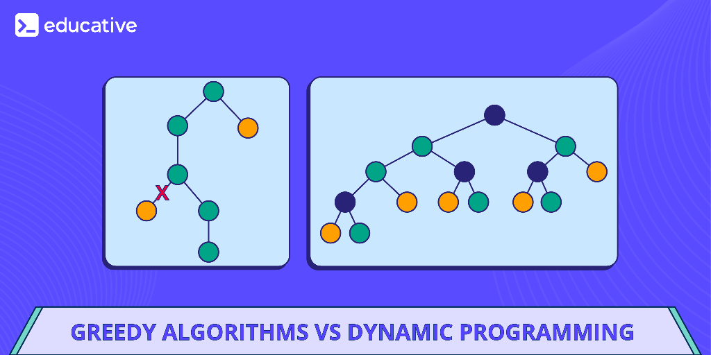
Greedy Algorithms vs. Dynamic Programming
Given your interest in Dynamic Programming (DP), it's crucial to distinguish it from the greedy approach.
| Feature | Greedy Algorithm | Dynamic Programming |
|---|---|---|
| Optimal Substructure | Yes, required. | Yes, required. |
| Greedy Choice Property | Yes, required. | Not required. |
| Decision Process | Makes a choice before solving subproblems. | Solves subproblems before making a choice. |
| Scope | Commits to one "best" choice, leading to one subproblem. | Explores all possible choices and their subproblems. |
| Nature | Top-down, one pass. Makes a choice and never reconsiders. | Typically bottom-up, building a table of subproblem solutions. |
A simple way to think about it:
- Greedy: Makes a choice, then solves the one subproblem that remains.
Choice -> Subproblem - Dynamic Programming: Solves all necessary subproblems, then makes a choice based on their solutions.
Subproblems -> Choice
Conclusion
In this lesson, we've established the theoretical bedrock for using greedy algorithms. You now have the tools to analyze a new problem and determine if a greedy approach is viable.
Key Takeaways:
- Greedy algorithms make a series of locally optimal choices to build a solution.
- For a greedy algorithm to be provably correct, the problem must have two properties:
- Optimal Substructure: An optimal solution to the problem contains optimal solutions to its subproblems.
- Greedy Choice Property: A locally optimal (greedy) choice is always part of some globally optimal solution. This is often proven with an "exchange argument."
- The key difference between Greedy and DP is that Greedy algorithms make their choice before solving the resulting single subproblem, while DP solves all subproblems first to figure out the best choice.
Preview of the Next Lesson:
Now that we understand the theory, it's time to put it into practice. In the next lesson, we will apply this framework to solve the Activity Selection Problem from start to finish. We'll formulate the greedy choice, implement the algorithm, and analyze its efficiency, solidifying the concepts we've covered today.