Duality in Linear Programming

1. An Intuitive Path to the Dual

Before jumping into formal definitions, let's understand why the dual exists. Imagine you have a maximization LP (the primal). You want to find the maximum possible value for your objective function. How could you be certain you've found it? One way is to find an upper bound on that value. The dual problem is, in essence, a systematic way of finding the best possible upper bound.

This video provides an excellent, step-by-step derivation of the dual by exploring this very idea of finding the tightest upper bound on a primal problem's objective value.

The core idea from the video is that we can multiply our primal constraints by some non-negative values $y_i$ and add them together. This creates a new, valid inequality. By choosing the $y_i$ values cleverly, we can make the left side of this new inequality look like an upper bound for our original objective function. The dual problem is simply the search for the $y_i$ values that make this upper bound as tight (i.e., as small) as possible.

2. The Duality Transformation: Standard Form

This intuitive process leads to a clean, mechanical transformation. Let's start with the standard form we defined in the last lesson. We'll call this the primal program.

Primal (Π)

Its corresponding dual program is constructed as follows:

Dual (⨿)

Notice the beautiful symmetry in this transformation:

• The maximization in the primal becomes a minimization in the dual.
• The primal objective coefficients $\mathbf{c}$ become the right-hand-side vector for the dual's constraints.
• The primal right-hand-side vector $\mathbf{b}$ becomes the objective coefficients for the dual.
• The constraint matrix $A$ is transposed to $A^T$.
• For each of the $m$ constraints in the primal, there is a corresponding dual variable $y_i$.
• For each of the $n$ variables in the primal, there is a corresponding dual constraint.

The document below provides a concise, formal definition of this relationship.

A key property highlighted in the reading is that duality is an involution: the dual of the dual is the original primal program. This means the choice of which to call "primal" is arbitrary; they are two sides of the same coin.

3. Duality for General Linear Programs

What if our primal LP is not in standard form? For example, what if it has equality constraints (=) or unrestricted variables? We could first convert it to standard form and then find the dual, but that can be tedious. A more direct method is to use a set of extended transformation rules.

The following video provides a systematic "recipe" for constructing the dual of any LP, regardless of its form.

The rules from the video can be summarized in a clear table. This table is your main tool for constructing duals.

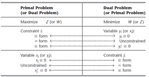
Let's walk through an example to solidify this. Consider the following primal LP:

Primal LP:

Let's construct its dual step-by-step using the rules:

1. Objective: The primal is max, so the dual will be min. The primal RHS vector is $\mathbf{b}=\left(\begin{array}{c}10\\ 4\end{array}\right)$. This becomes the dual objective coefficients.

   • Dual Objective: minimize 10y_1 + 4y_2

2. Dual Variables: The primal has two constraints, $C_1$ and $C_2$, so the dual will have two variables, $y_1$ and $y_2$.

   • Primal constraint $C_1$ is an equality (=). The table tells us the corresponding dual variable, $y_1$, is unrestricted.
   • Primal constraint $C_2$ is a less-than-or-equal-to (≤). The table tells us the corresponding dual variable, $y_2$, is non-negative (≥ 0).

3. Dual Constraints: The primal has two variables, $x_1$ and $x_2$, so the dual will have two constraints. The primal objective coefficients are $\mathbf{c}=\left(\begin{array}{c}5\\ 6\end{array}\right)$, which become the dual RHS. The primal constraint matrix $A=\left(\begin{array}{cc}1& 2\\ 2& -1\end{array}\right)$ is transposed to $A^T=\left(\begin{array}{cc}1& 2\\ 2& -1\end{array}\right)$.

   • The first dual constraint corresponds to primal variable $x_1$. Since $x_1\ge 0$, this dual constraint will be a greater-than-or-equal-to (≥) type. The coefficients are from the first column of $A$ (or first row of $A^T$).
     • 1*y_1 + 2*y_2 ≥ 5
   • The second dual constraint corresponds to primal variable $x_2$. Since $x_2$ is unrestricted, this dual constraint will be an equality (=). The coefficients are from the second column of $A$ (or second row of $A^T$).
     • 2*y_1 - 1*y_2 = 6

Putting it all together, we get the complete dual LP.

Dual LP:

Conclusion

In this lesson, we demystified the concept of the dual linear program. We saw that it arises naturally from the search for the tightest upper bound on a primal problem's solution, and we established a set of mechanical rules to construct it for any given LP.

Key Takeaways:

• Every linear program (the primal) has a corresponding dual program.
• For a standard max primal, the dual is a min problem where the roles of the objective coefficients ($\mathbf{c}$) and the constraint bounds ($\mathbf{b}$) are swapped. The constraint matrix is transposed ($A^T$).
• There is a precise symmetry between the types of constraints in the primal and the sign restrictions on the variables in the dual, and vice-versa.
• This relationship allows us to construct the dual for any LP, not just those in standard form.

Preview of the next lesson:

Now that we can construct both a primal and a dual LP, the natural question is: what is the exact relationship between their solutions? In the next lesson, we will state and prove the Weak Duality Theorem. This theorem formalizes the intuition we started with today—that the objective value of any feasible solution to a dual min problem provides an upper bound for the objective value of any feasible solution to its corresponding primal max problem. This is the first major step in connecting LP duality to the Minimax Theorem.