Introduction
Hello! In our previous lessons, we've built a solid toolkit for unsupervised learning. You've learned how to use K-means to find hidden groups in data and how to use Principal Component Analysis (PCA) to reduce high-dimensional data into a more manageable, lower-dimensional representation. You saw how PCA can project a dataset with dozens of features onto a simple 2D plane, capturing the most important variance.
Today, we will combine these two powerful techniques. Our learning outcome is to visualize the results of clustering on a 2D projection of data created with PCA. When you perform clustering on data with more than three features, it's impossible to "see" the clusters you've found. This lesson will show you how to use PCA to create an informative 2D "shadow" of your data and then color it in to reveal the structure of your high-dimensional clusters. This is one of the most common and insightful applications in data analysis.
Part 1: The Main Workflow for Visualizing Clusters
The primary goal is to understand the structure of clusters found in high-dimensional space. The most direct way to achieve this involves two parallel processes: one for clustering and one for visualization.
Here is the step-by-step workflow:
- Scale the Data: As always, start with your high-dimensional, scaled dataset.
- Perform Clustering: Run the K-means algorithm on the full, high-dimensional scaled data. This process assigns a cluster label to every data point based on all the available information.
- Perform PCA for Visualization: In a separate step, take the same scaled dataset and use PCA to reduce its dimensionality down to exactly two components (Principal Component 1 and Principal Component 2).
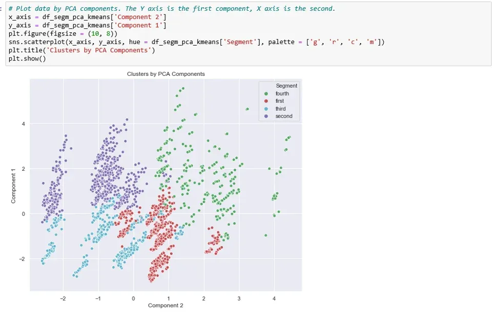
- Plot the Results: Create a 2D scatter plot. The x-axis will be Principal Component 1, and the y-axis will be Principal Component 2. For each point on the plot, use the cluster label you found in Step 2 to assign its color.
This process effectively answers the question: "If I could see my 30-dimensional data, what would the clusters I found look like?"
The following article provides a fantastic walkthrough of this exact workflow. Pay close attention to how it uses the cluster labels to color the PCA plot.
Friendly k-means and PCA python tutorial
The article 'Friendly k-means and PCA python tutorial' from Step By Step Data Science clearly demonstrates this visualization technique.
Please read the section titled 'Earlier we saw how we could plot our data using the first two principal components. Now we can do the same but this time we can colour the points to match their cluster:'. Study the text and the accompanying image ('py PCA cluster plot.png'). Focus on how the visualization brings the abstract cluster assignments to life on a 2D plane.
As you saw in the article, this visualization immediately makes the clustering results interpretable. You can see which clusters are distinct, which overlap, and how they are distributed along the axes of maximum variance.
Here is a typical implementation of this workflow in Python:
# Assume X_scaled is our high-dimensional scaled data

from sklearn.cluster import KMeans
from sklearn.decomposition import PCA
import matplotlib.pyplot as plt
import seaborn as sns


# Step 1: Perform K-means clustering on the full, high-dimensional data
kmeans = KMeans(n_clusters=4, n_init=10, random_state=42)
cluster_labels = kmeans.fit_predict(X_scaled)


# Step 2: Perform PCA to reduce the data to 2 dimensions for visualization
pca = PCA(n_components=2)
X_pca = pca.fit_transform(X_scaled)


# Step 3: Create a DataFrame with PCA results and cluster labels
import pandas as pd
pca_df = pd.DataFrame(data=X_pca, columns=['Principal Component 1', 'Principal Component 2'])
pca_df['Cluster'] = cluster_labels


# Step 4: Visualize the clusters
plt.figure(figsize=(12, 8))
sns.scatterplot(x='Principal Component 1', y='Principal Component 2', hue='Cluster',
                palette='viridis', data=pca_df, alpha=0.7)
plt.title('K-Means Clusters Visualized with PCA')
plt.show()
This resulting plot gives you a powerful summary of your unsupervised learning analysis.
Part 2: An Alternative Workflow — PCA as a Preprocessing Step
There is another common way to combine PCA and K-means. Instead of just using PCA for visualization, you can use it to preprocess the data before clustering.
The logic behind this approach is that high-dimensional data can suffer from the "curse of dimensionality," where distance metrics become less meaningful. It can also be noisy and contain redundant (correlated) features. By first applying PCA, you can:
- Reduce noise by discarding components that explain little variance.
- Create a new set of uncorrelated features (the principal components).
- Potentially improve the speed and quality of the clustering algorithm.
The workflow looks like this:
- Scale the Data.
- Perform PCA for Dimensionality Reduction: Reduce the data to a smaller, but still meaningful, number of components (e.g., the number needed to explain 80% or 90% of the variance). This might be 5, 10, or more components, not necessarily just 2.
- Perform Clustering: Run K-means on the new, lower-dimensional data from Step 2.
- Visualize: Create a scatter plot using only the first two principal components from the PCA-transformed data (from Step 2) and color the points using the cluster labels found in Step 3.
The following video provides an excellent, code-heavy walkthrough of this entire process.
370 - Principal Component Analysis (PCA): Mastering Dimensionality Reduction & Visualization
The video 'Principal Component Analysis (PCA): Mastering Dimensionality Reduction & Visualization' by DigitalSreeni demonstrates using PCA as a preprocessing step before applying K-means.
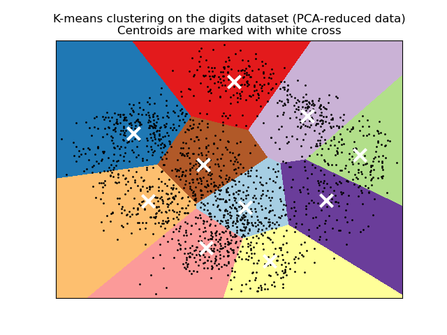
Watch the segment from 33:47 to 40:22. This is a dense section, so feel free to pause and re-watch. The presenter performs the following key steps: Applies PCA to the scaled data to reduce it to 2 components. Runs K-means clustering directly on this 2D PCA-transformed data. Visualizes the resulting clusters and the algorithm's decision boundary on the 2D plot. Notice the crucial difference: the clustering happens on the PCA data, not the original high-dimensional data.
Comparing the Two Workflows
You've now seen two valid ways to combine PCA and K-means. Let's clarify the distinction:
-
Workflow 1 (Visualize After):
Data -> K-Means. ThenData -> PCA -> Plot.- Purpose: Purely for visualization.
- Pros: The clusters are found using all the information in the original dataset. The visualization is a faithful projection of these "true" clusters.
- Cons: Clustering can be slow or less effective on very high-dimensional, noisy data.
-
Workflow 2 (Preprocess Before):
Data -> PCA -> K-Means -> Plot.- Purpose: Preprocessing to improve clustering, followed by visualization.
- Pros: Can lead to faster and sometimes better-defined clusters by removing noise and redundancy.
- Cons: The clusters are based on a reduced-information version of the data. You are trading some information for computational efficiency and noise reduction.
In practice, both are useful. Often, the clusters found by both methods are very similar. In that case, the first workflow often provides a more straightforward story, as the clusters can be explained using the original features. The second workflow is particularly powerful when dealing with extremely high-dimensional data (e.g., thousands of features).
To reinforce what the final output looks like, here is a classic example from the scikit-learn documentation.
Conclusion
In this lesson, you've learned how to bring together dimensionality reduction and clustering to create insightful visualizations. This is a cornerstone of exploratory data analysis in machine learning.
Key Takeaways:
- PCA is the primary tool for visualizing the results of clustering on high-dimensional data.
- The main workflow involves clustering on the full data and then using PCA to create a 2D plot, coloring the points by their cluster labels.
- An alternative workflow uses PCA as a preprocessing step to reduce dimensionality before running K-means, which can improve performance and reduce noise.
- The final scatter plot, with axes of Principal Component 1 and 2, reveals the structure, separation, and overlap of the clusters you've identified.
Preview of the Next Lesson:
We are now concluding our module on Unsupervised Learning. You have a firm grasp of clustering and dimensionality reduction. In our next module, we will enter the world of Neural Networks. The first lesson, "Describe the structure of a single artificial neuron, including weights, bias, and activation function," will introduce you to the fundamental building block of modern AI, setting the stage for building the powerful deep learning models that drive today's most advanced applications.