Understanding Multi-Layer Feedforward Neural Network Architecture

From Neurons to Networks: The Layered Structure

A neural network organizes its neurons into a series of layers. Information flows in one direction—from the first layer to the last—which is why it's called a feed-forward network.

To build a strong intuition for this structure, let's start with a classic video from 3Blue1Brown. It uses the problem of recognizing handwritten digits to motivate why we need layers and what role each one plays.

As the video illustrated, a typical feed-forward network has three types of layers:

1. Input Layer: The entry point of the network.
2. Hidden Layers: The intermediate layers where most of the computation occurs.
3. Output Layer: The final layer that produces the result or prediction.

The Anatomy of a Feed-Forward Network

Let's formally define the architecture and its components. The most common type of feed-forward network used in practice is the Multi-Layer Perceptron (MLP).

A common point of confusion is the relationship between FFNNs and MLPs. Let's clarify that.

So, for our purposes, when we talk about a multi-layer feedforward network, we are describing an MLP. Let's look at its structure.

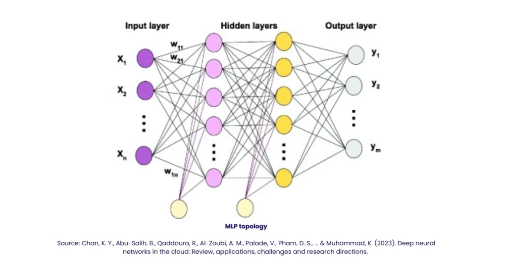
This structure is defined by a few key terms that come from the more formal academic literature.

To summarize and solidify these concepts:

• Layers: The network is organized into an input layer, one or more hidden layers, and an output layer.
• Fully Connected (or Dense): In an MLP, each neuron in a given layer is connected to every neuron in the next layer. This is what the web of lines in the diagram represents.
• Depth: The number of layers in the network. "Deep learning" refers to training networks with many layers (i.e., great depth).
• Width: The number of neurons in a particular layer.

The Role of Each Layer

Now that we have the terminology, let's clarify the specific job of each layer type.

Here's a breakdown based on that reading:

• Input Layer: This layer doesn't perform any computation. Its neurons simply act as entry points, holding the values of the input features. For an image, this would be the pixel values; for predicting house prices, it might be features like square footage and number of bedrooms. The width of this layer is determined by the number of features in your dataset.

• Hidden Layers: This is where the learning happens. Each neuron in a hidden layer receives outputs from all neurons in the previous layer. It then performs the calculation you're familiar with:

  1. Computes a weighted sum of its inputs.
  2. Adds a bias.
  3. Applies a non-linear activation function (like ReLU, which we discussed previously).
     The outputs of these neurons are then passed as inputs to the next layer. Through training, the weights and biases of these hidden layers are adjusted so the neurons learn to detect increasingly complex patterns.

• Output Layer: This final layer produces the network's prediction. As we covered in the last lesson, its design is tailored to the specific problem:

  • Regression: Typically one neuron with a linear (or no) activation to predict a continuous value.
  • Binary Classification: One neuron with a sigmoid activation to output a probability between 0 and 1.
  • Multi-class Classification: One neuron per class with a softmax activation to output a probability distribution across all classes.

The Mathematics of Information Flow

We've described the static architecture. Now, let's formalize how data flows through it. The process is a sequence of matrix operations, which is why having some familiarity with linear algebra is so helpful.

The 3Blue1Brown video provides a fantastic conceptual bridge from the visual idea of connections to the underlying mathematics.

The video demonstrates that the activation of a single neuron is a weighted sum of the previous layer's activations, plus a bias, all passed through an activation function. When you consider all the neurons in a layer, this entire set of calculations can be written as a single, clean equation using matrix multiplication.

Let's look at the formal mathematical notation. Given your background, seeing the equations laid out will help solidify the theory.

To recap the vectorized notation, the activation vector of a layer, ${\mathbf{h}}^{(\ell )}$, is computed from the activation vector of the previous layer, ${\mathbf{h}}^{(\ell -1)}$, as follows:

Where:

• ${\mathbf{h}}^{(\ell )}$ is the vector of activations for layer $\ell$.
• $\varphi$ is the activation function (e.g., ReLU), applied element-wise.
• ${\mathbf{W}}^{(\ell )}$ is the weight matrix for layer $\ell$, where each entry $W_{ij}$ is the weight from neuron $j$ in the previous layer to neuron $i$ in the current layer.
• ${\mathbf{b}}^{(\ell )}$ is the bias vector for layer $\ell$.

This elegant equation describes the entire transformation from one layer to the next. The whole network is just a chain of these transformations.

Conclusion

In this lesson, we moved from the single neuron to the complete architecture of a multi-layer feedforward neural network (MLP). You now have the blueprint for the fundamental structure used in a vast range of AI applications.

Key Takeaways:

• A feed-forward neural network processes data in one direction through a series of layers: an input layer, one or more hidden layers, and an output layer.
• An MLP is a "fully connected" network, meaning every neuron in one layer connects to every neuron in the next.
• The input layer holds the initial data, the hidden layers perform non-linear transformations to learn complex features, and the output layer produces the final prediction.
• The entire process of information flowing from one layer to the next can be expressed efficiently using matrix and vector operations, forming the core computation of the network.

Preview of the Next Lesson:
We have now described the static architecture and the mathematical formula for one layer's computation. In the next lesson, we will put this into motion. We will explain the process of forward propagation, which is the step-by-step procedure of taking a single input, passing it through the entire network, layer by layer, to generate a final prediction.