Gradient Descent: A Manual Walkthrough

1. The Core Concept and Algorithm

Imagine you're standing on a foggy hill and want to get to the lowest point. You can't see the whole valley, but you can feel the slope right under your feet. The most straightforward strategy is to:

1. Check the direction of the steepest downhill slope.
2. Take a small step in that direction.
3. Repeat the process from your new position.

Gradient descent is the mathematical formalization of this exact process. It's an iterative algorithm that takes successive steps "downhill" on a function's surface to find a minimum.

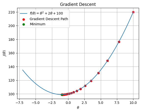
The algorithm itself is defined by a simple update rule. To find the next position, $x_{k+1}$, we start from our current position, $x_k$, and subtract the scaled gradient.

To understand the formal steps and the components of this rule, let's turn to a clear textual explanation.

As the article explains, the update rule for a single-variable function $f(x)$ is:

Let's break down the components:

• $x_k$ is our current position at step $k$.
• $x_{k+1}$ is the next position we are calculating.
• $f^{\prime }(x_k)$ is the derivative (gradient) of the function evaluated at our current position. This tells us the direction of the steepest slope.
• $\eta$ (the Greek letter 'eta') is the learning rate. It's a small positive number (e.g., 0.1, 0.01) that controls how big of a step we take. This is a crucial parameter you'll encounter constantly in machine learning.

The overall process is:

1. Choose a random starting point, $x_0$.
2. Choose a learning rate, $\eta$.
3. Repeat for a set number of iterations:
   • Calculate the derivative at the current point: $f^{\prime }(x_k)$.
   • Update the position using the rule: $x_{k+1}=x_k-\eta \cdot f^{\prime }(x_k)$.

2. A Worked Example: Step-by-Step Calculation

Now that you understand the theory, let's apply it. We'll walk through the first few iterations of gradient descent for a simple quadratic function. This hands-on process is exactly what this lesson is about.

The following video provides a clear, step-by-step calculation for finding the minimum of a function.

Let's formalize the steps from the video on paper to ensure the process is clear.

Problem Setup:

• Function: $f(x)=(x+5{)}^2$. By looking at the function, we know the minimum occurs when the squared term is zero, i.e., at $x=-5$. Let's see if gradient descent can find it.
• Derivative: Using the chain rule, $f^{\prime }(x)=2\cdot (x+5{)}^1\cdot 1=2(x+5)$.
• Initial Point: $x_0=-3$.
• Learning Rate: $\eta =0.01$.

Iteration 1:

1. Calculate the gradient at $x_0$:

   $$f^{\prime }(x_0)=f^{\prime }(-3)=2(-3+5)=2(2)=4$$

   A positive gradient means the slope is upwards, so we need to move to the left (decrease x) to go downhill.

2. Apply the update rule:

   $$x_1=x_0-\eta \cdot f^{\prime }(x_0)=-3-(0.01\cdot 4)=-3-0.04=-3.04$$

After one step, we've moved from $x=-3$ to $x=-3.04$, which is closer to the true minimum of -5.

Iteration 2:

1. Calculate the gradient at our new point, $x_1$:

   $$f^{\prime }(x_1)=f^{\prime }(-3.04)=2(-3.04+5)=2(1.96)=3.92$$

   The gradient is still positive but slightly smaller, meaning the slope is less steep.

2. Apply the update rule:

   $$x_2=x_1-\eta \cdot f^{\prime }(x_1)=-3.04-(0.01\cdot 3.92)=-3.04-0.0392=-3.0792$$

After two steps, we are at $x=-3.0792$, even closer to the minimum. We would continue this process until the change in $x$ becomes very small, indicating we've arrived at the bottom of the valley.

3. Practice and the Importance of the Learning Rate

Let's try another example to solidify your understanding.

As you've seen, the choice of the learning rate, $\eta$, is critical.

• If $\eta$ is too small: The algorithm will take tiny steps and converge very slowly, potentially running out of time (or iterations) before reaching the minimum.
• If $\eta$ is too large: The algorithm might "overshoot" the minimum, jumping from one side of the valley to the other. In worse cases, it can cause the steps to get larger and larger, making the algorithm diverge completely.

To visualize this effect, let's explore a resource that demonstrates what happens with different learning rates.

Finding the right learning rate is a key part of training machine learning models and is often done through experimentation.

Conclusion

You have now successfully performed the single most fundamental optimization procedure in AI. By working through the calculations on paper, you've built a robust mental model of how a system can "learn" to find the best configuration by minimizing an error function.

Key Takeaways:

• Gradient Descent is an iterative optimization algorithm used to find the minimum of a function.
• The core principle is to take small, repeated steps in the direction opposite to the gradient ($-\nabla f$).
• The update rule for a single-variable function is $x_{k+1}=x_k-\eta \cdot f^{\prime }(x_k)$.
• The learning rate ($\eta$) is a critical hyperparameter that controls step size. A value that is too large can cause divergence, while one that is too small can lead to slow convergence.

Preview of the Next Lesson:
Manually calculating these steps is excellent for understanding the process, but it's not practical for the thousands or millions of iterations needed to train a real model. In the next lesson, "Implement gradient descent in Python for a single-variable function," we will take the exact algorithm you learned today and write a program to do the work for us. This will be your first step in translating foundational AI theory into practical, working code.