Matrix-Vector Multiplication

1. The Core Idea: Matrices as Transformations

Before we jump into the mechanics of multiplication, it's crucial to build a strong mental model of what matrix multiplication does. The most powerful way to think about a matrix is as a function that performs a linear transformation. It takes an input vector and produces an output vector, effectively moving it to a new location in space.

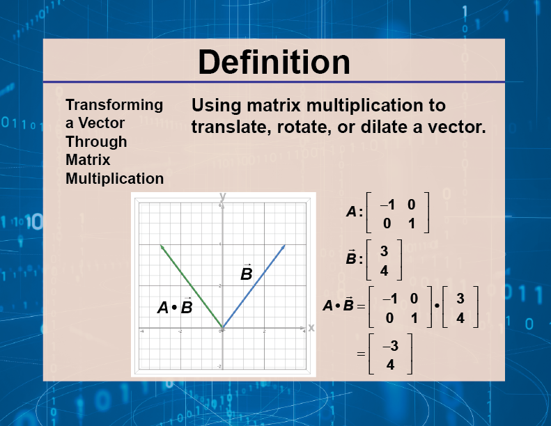
What makes a transformation "linear"? Visually, it's a transformation that keeps grid lines parallel and evenly spaced, and the origin stays put. To see this in action and understand how this geometric idea connects to the numbers in a matrix, let's watch one of the most insightful videos on the topic.

The crucial takeaway from the video is this: the product of a matrix $\mathbf{A}$ and a vector $\mathbf{x}$, written as $\mathbf{Ax}$, is the resulting vector after applying the linear transformation described by $\mathbf{A}$ to $\mathbf{x}$.

2. Matrix-Vector Multiplication: Two Perspectives

Now that we have the conceptual foundation, let's look at the two main ways to compute the product $\mathbf{Ax}$. Both give the same result but offer different insights.

Perspective 1: A Linear Combination of Columns

This perspective flows directly from the 3Blue1Brown video. If the columns of matrix $\mathbf{A}$ represent the transformed basis vectors, then the product $\mathbf{Ax}$ is simply a linear combination of those columns, where the components of vector $\mathbf{x}$ act as the scalars (the weights).

In the previous lesson, you learned that a linear combination is a sum of scaled vectors, like $c_1{\mathbf{v}}_1+c_2{\mathbf{v}}_2$. Matrix-vector multiplication is exactly that.

Let's say $\mathbf{A}$ has columns ${\mathbf{a}}_1,{\mathbf{a}}_2,\dots ,{\mathbf{a}}_n$ and $\mathbf{x}$ has components $x_1,x_2,\dots ,x_n$. Then:

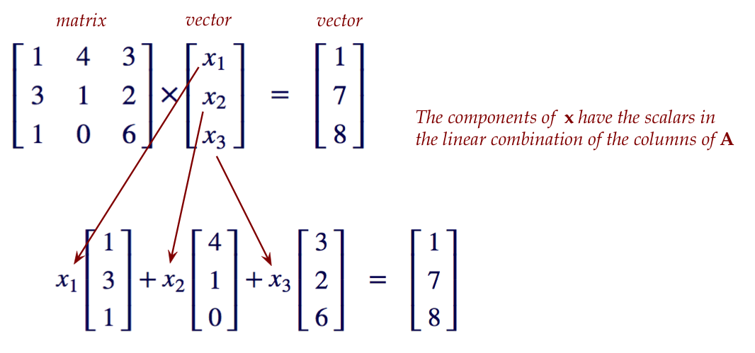
This view is incredibly powerful for understanding what a matrix "does" to a vector.

Perspective 2: The Row-Column Dot Product

This is the standard, mechanical method taught in most textbooks. It's less intuitive but essential for computation by hand and for understanding the structure of the calculation.

To get the i-th element of the resulting vector, you compute the dot product of the i-th row of the matrix $\mathbf{A}$ with the column vector $\mathbf{x}$.

Let's solidify both perspectives with a clear, visual guide.

Before moving on, make sure you can answer:

1. If I give you a 2x2 matrix and a 2D vector, can you calculate the result using the linear combination of columns?
2. Can you calculate the same result using the row-column dot product method?

3. Matrix-Matrix Multiplication: Composing Transformations

What happens when we multiply two matrices, $\mathbf{C}=\mathbf{AB}$?

Conceptually, this corresponds to composing two linear transformations. First, you apply the transformation of $\mathbf{B}$, and then you apply the transformation of $\mathbf{A}$ to that result. For example, $\mathbf{B}$ could be a rotation, and $\mathbf{A}$ could be a shear. The product matrix $\mathbf{C}=\mathbf{AB}$ is a new, single matrix that represents the net effect of doing the rotation then the shear.

This gives us an intuitive way to calculate the product, which builds directly on what we just learned.

Perspective 3: A Matrix Acting on Columns

We can view the matrix $\mathbf{B}$ as a collection of column vectors. The product $\mathbf{AB}$ is found by multiplying the matrix $\mathbf{A}$ with each column of $\mathbf{B}$ individually. The resulting vectors become the columns of the new matrix $\mathbf{C}$.

If $\mathbf{B}=[{\mathbf{b}}_1|{\mathbf{b}}_2|\dots |{\mathbf{b}}_p]$, then:

Each $\mathbf{A}{\mathbf{b}}_j$ is a standard matrix-vector multiplication, which you already know how to do.

Of course, the standard row-column dot product method also extends to matrix-matrix multiplication. The entry in the i-th row and j-th column of the product matrix $\mathbf{C}$ is the dot product of the i-th row of $\mathbf{A}$ and the j-th column of $\mathbf{B}$.

Let's see how this works in practice.

Now let's see the standard calculation and the implementation in NumPy.

A crucial property to internalize is that matrix multiplication is not commutative. In general, $\mathbf{AB}\ne \mathbf{BA}$. Geometrically, this makes perfect sense: performing a rotation then a shear is not the same as performing a shear then a rotation. The order of transformations matters.

Conclusion

In this lesson, we demystified matrix multiplication, elevating it from a mechanical recipe to a deep conceptual tool. You now have the ability to not just compute, but also interpret, the product of matrices and vectors.

Key Takeaways:

• Matrix as Transformation: A matrix is best understood as an object that performs a linear transformation on space.
• Matrix-Vector Product: The product $\mathbf{Ax}$ is the new vector that results from applying transformation $\mathbf{A}$ to vector $\mathbf{x}$. It can be computed as a linear combination of $\mathbf{A}$'s columns or through row-column dot products.
• Matrix-Matrix Product: The product $\mathbf{AB}$ represents the composition of two transformations. It can be computed by applying $\mathbf{A}$ to each column of $\mathbf{B}$.
• Non-Commutativity: The order of matrix multiplication matters ($\mathbf{AB}\ne \mathbf{BA}$), because the order of transformations matters.
• Implementation: In Python, NumPy's np.dot(A, B) or the @ operator (A @ B) are used to perform this operation efficiently.

Preview of the Next Lesson:
Today, you learned the powerful idea that a matrix represents a transformation. In the next lesson, we will flip this around. We will start with a desired geometric transformation—like a specific rotation, scaling, or shear—and your goal will be to describe these linear transformations by constructing the specific matrices that produce them. This will complete the loop, giving you full command over the relationship between the numbers in a matrix and their geometric effect on data.