Analyzing Space Complexity: Auxiliary Space and Recursion

1. What is Space Complexity?

Just as time complexity measures how runtime grows, space complexity measures how the amount of memory an algorithm needs grows as the input size (n) increases. Like time complexity, we use Big O notation to describe this growth.

An algorithm's total memory usage can be broken down into two parts:

• Input Space: The memory required to store the input data itself (e.g., an array of size n).
• Auxiliary Space: The extra or temporary memory that an algorithm uses during its execution. This includes variables, data structures created to aid the computation, and the space used by function calls.

Space Complexity = Input Space + Auxiliary Space

In many interview contexts and competitive programming, when someone asks for "space complexity," they are often most interested in the auxiliary space complexity. Why? Because the input space is a given requirement of the problem, while the auxiliary space is a direct consequence of your algorithmic choices. A solution with O(1) auxiliary space is generally better than one with O(n) auxiliary space, even if both have the same total space complexity of O(n).

2. Analyzing Space in Iterative Algorithms

Let's analyze some familiar iterative code to see how this works.

Example 1: Constant Auxiliary Space, O(1)

Consider a function that sums the elements of an array.

// arr has n elements
long sumArray(int[] arr) {
    long sum = 0; // One variable (e.g., 8 bytes)
    // The loop counter 'i' is also one variable (e.g., 4 bytes)
    for (int i = 0; i < arr.length; i++) {
        sum += arr[i];
    }
    return sum;
}

• Input Space: The array arr takes O(n) space.
• Auxiliary Space: We use two variables, sum and i. The memory they occupy does not change, regardless of whether the array has 10 elements or 10 million. This is constant space, which we denote as O(1).
• Total Space Complexity: O(n) (input) + O(1) (auxiliary) = O(n).

Example 2: Linear Auxiliary Space, O(n)

Now, let's look at a function that creates a new data structure. Imagine we want to count the frequency of each number in an array. A HashMap is a good tool for this.

Let's analyze the code from the article:

static void countFreq(int arr[], int n) {
    // Auxiliary space starts here
    HashMap<Integer, Integer> freq = new HashMap<>();

    for (int i = 0; i < n; i++) {
        // The map grows as we add elements
        freq.put(arr[i], freq.getOrDefault(arr[i], 0) + 1);
    }
    // ...
}

• Input Space: The array arr takes O(n) space.
• Auxiliary Space: We create a HashMap called freq. In the worst-case scenario (where all n elements in arr are unique), the map will store n key-value pairs. Therefore, the space required by the map grows linearly with the input size. The auxiliary space is O(n).
• Total Space Complexity: O(n) (input) + O(n) (auxiliary) = O(n).

Notice that while both examples have O(n) total space complexity, their auxiliary space requirements are vastly different. This is the kind of trade-off you'll constantly evaluate.

int[] getSquares(int[] nums) {
    int n = nums.length;
    int[] squares = new int[n]; // A new array is created
    for (int i = 0; i < n; i++) {
        squares[i] = nums[i] * nums[i];
    }
    return squares;
}

An Important Rule for Interviews

It can be tempting to save space by modifying the input data directly. For example, in the getSquares problem above, you could overwrite nums[i] with its square. While this reduces auxiliary space to O(1), it's generally considered bad practice unless you're explicitly told it's acceptable.

3. Space Complexity of Recursive Algorithms: The Call Stack

Analyzing space in recursive algorithms requires understanding the call stack. When a function is called, a block of memory called a stack frame is allocated to store its local variables, parameters, and return address. When functionA calls functionB, a new stack frame for functionB is pushed on top of functionA's frame.

The space complexity of a recursive algorithm is determined by the maximum depth of the call stack at any point during execution.

Example 1: Linear Space Recursion, O(n)

Let's revisit the factorial function from the last lesson.

int factorial(int n) {
    if (n <= 1) {
        return 1;
    }
    return n * factorial(n - 1);
}

When you call factorial(4), the call stack looks like this before the base case is hit:

1. factorial(4) is called.
2. factorial(4) calls factorial(3). Stack: [factorial(4), factorial(3)]
3. factorial(3) calls factorial(2). Stack: [factorial(4), factorial(3), factorial(2)]
4. factorial(2) calls factorial(1). Stack: [factorial(4), factorial(3), factorial(2), factorial(1)]

The stack reaches its maximum depth of n (or n+1 depending on how you count). Since each stack frame takes O(1) space, the total space complexity due to recursion is O(n).

Example 2: Time vs. Space in Branching Recursion

In the last lesson, we saw that the fibonacci function has a time complexity of O(2^n) because of its branching recursion tree. What about its space complexity?

int fibonacci(int n) {
    if (n <= 1) {
        return n;
    }
    return fibonacci(n - 1) + fibonacci(n - 2); 
}

Although the total number of calls is exponential, they don't all exist on the call stack at the same time. The program explores one branch of the recursion tree down to its base case, and only then does it backtrack to explore another. The maximum number of stack frames on the call stack at any single moment is determined by the height of the recursion tree, which is n.

Therefore, the space complexity of this fibonacci function is O(n), not O(2^n). This is a critical distinction and a common interview question.

Example 3: Logarithmic Space Recursion, O(log n)

What happens if a recursive call halves the problem size, like in a recursive binary search?

// A simplified recursive function that divides its input
void function(int n) {
    if (n <= 1) {
        return; // Base case
    }
    function(n / 2); // Recurse on half the problem
}

The sequence of calls would be n -> n/2 -> n/4 -> ... -> 1. The number of times you can divide n by 2 until you reach 1 is log₂(n). The maximum depth of the call stack is log n. Therefore, the space complexity is O(log n).

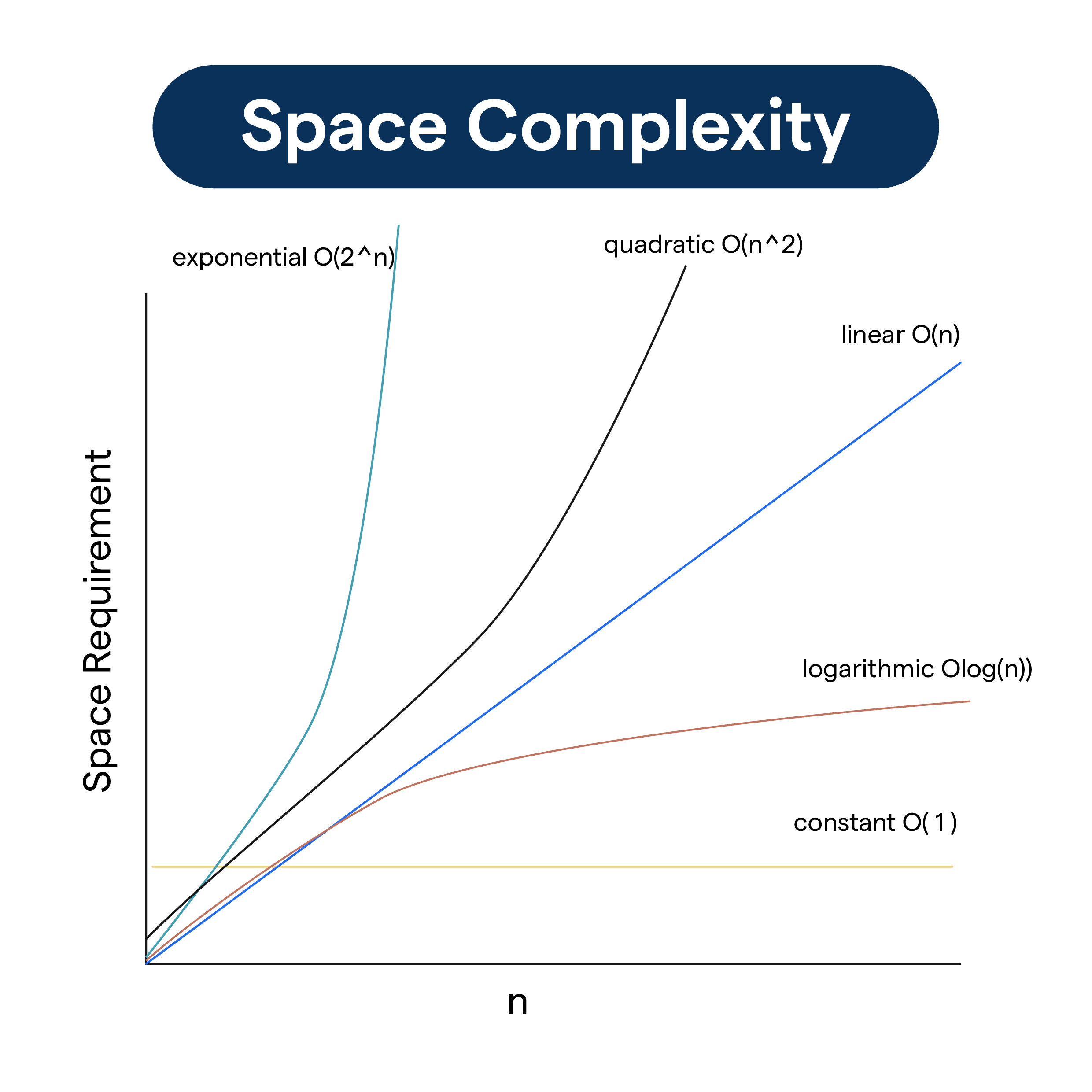
Visualizing Space Complexity

Just like with time complexity, we can visualize how different space complexities scale. Efficient algorithms aim for lower space requirements, especially as the input size n grows large.

int recursiveSum(int[] arr, int index) {
    // Base case
    if (index == arr.length) {
        return 0;
    }
    // Recursive step
    return arr[index] + recursiveSum(arr, index + 1);
}

Conclusion

You have now completed your tour of the fundamentals of algorithm analysis. You can analyze an algorithm's efficiency in terms of both time and space, for both iterative and recursive solutions. This two-dimensional perspective is essential for making informed decisions as a software engineer and for succeeding in technical interviews.

Key Takeaways:

• Space Complexity measures an algorithm's memory usage as a function of input size n.
• Auxiliary Space is the extra memory used by an algorithm, distinct from the input space. This is often the primary focus of analysis.
• Iterative Algorithms: Space is determined by the variables and data structures you declare. This can be O(1), O(n), or other complexities.
• Recursive Algorithms: Space is primarily determined by the maximum depth of the call stack. Linear recursion is typically O(n), while "divide and conquer" recursion is often O(log n).
• Time vs. Space: A branching recursion like Fibonacci can have exponential time (O(2^n)) but linear space (O(n)).

Preview of the next lesson:
Now that you have the tools to analyze algorithms, we will begin learning specific techniques to design efficient ones. In the next lesson, we will cover the Two-Pointer Technique, a simple yet powerful pattern for solving a wide range of problems on arrays and strings in optimal time and space.