Finding the Lowest Common Ancestor (LCA)

1. What is a Lowest Common Ancestor?

The Lowest Common Ancestor (LCA) between two nodes, p and q, in a binary tree is the lowest (deepest) node that has both p and q as descendants. A key part of this definition is that a node can be a descendant of itself.

Let's look at a simple example.

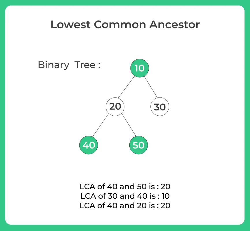
This problem appears in various contexts, from calculating distances between nodes in a network to version control systems like Git finding a common base for merging branches.

2. Approach 1: Storing Root-to-Node Paths

An intuitive way to solve this is to think about the paths from the root to each of our target nodes.

1. Find the path from the root to node p and store it in a list.
2. Find the path from the root to node q and store it in another list.
3. Compare these two paths. The last node they have in common is the LCA.

For a detailed explanation of this method, including how to implement the path-finding logic, please read the following resource.

This method works correctly, but it has some drawbacks:

• Time Complexity: You need to traverse the tree to find the first path and then again for the second path. This leads to a time complexity of $O(N)$, as in the worst case you might visit all nodes.
• Space Complexity: You need to store the paths. In the worst case of a skewed tree, a path could be as long as the number of nodes, leading to a space complexity of $O(N)$ (or $O(H)$ where H is the height of the tree).

Given your goal of preparing for competitive programming and technical interviews, it's essential to know a more optimized solution that uses less space and only requires a single traversal of the tree.

3. Approach 2: The Efficient Single-Pass Recursion

The most elegant and efficient solution uses recursion to find the LCA in a single traversal. The core idea is to define a recursive function that searches for p and q in the subtrees and uses the return values to pinpoint the LCA.

To understand the logic, let's watch a short video that introduces the concept and the algorithm.

The Recursive Logic

The recursive function lowestCommonAncestor(root, p, q) has a clear "contract". It returns:

• The node itself (root), if root is null or if root is one of the nodes we're looking for (p or q).
• The actual LCA, if p and q are found in different subtrees of the current root.
• A non-null node, if both p and q are found in the same subtree of the root.
• null, if neither p nor q can be found in the tree rooted at root.

This translates into a simple, powerful algorithm:

1. Base Case: If the current node (root) is null, or if it matches p or q, return root. Finding p or q is a success condition, so we propagate that node up the call stack.
2. Recursive Step: Recursively call the function for the left and right children:
   • TreeNode leftLCA = lowestCommonAncestor(root.left, p, q);
   • TreeNode rightLCA = lowestCommonAncestor(root.right, p, q);
3. Analyze Results: After the recursive calls return, analyze leftLCA and rightLCA:
   • If leftLCA and rightLCA are both not null, it means p was found in the left subtree and q was found in the right subtree (or vice-versa). Therefore, the current root is the split point and the LCA. We return root.
   • If only leftLCA is not null, it means both p and q are in the left subtree. The leftLCA that was returned is the actual LCA. So, we return leftLCA.
   • Similarly, if only rightLCA is not null, we return rightLCA.
   • If both are null, neither node was found in this subtree, so we return null.

To see this logic in action, let's watch a detailed walkthrough.

Java Implementation

Here is the Java implementation, which beautifully reflects the concise logic we just discussed.

/**
 * Definition for a binary tree node.
 * public class TreeNode {
 *     int val;
 *     TreeNode left;
 *     TreeNode right;
 *     TreeNode(int x) { val = x; }
 * }
 */
class Solution {
    public TreeNode lowestCommonAncestor(TreeNode root, TreeNode p, TreeNode q) {
        // Base case: if root is null, or we've found p or q, return the root.
        if (root == null || root == p || root == q) {
            return root;
        }

        // Recur for left and right subtrees
        TreeNode leftLCA = lowestCommonAncestor(root.left, p, q);
        TreeNode rightLCA = lowestCommonAncestor(root.right, p, q);

        // If both subtrees returned a non-null node, then the current root is the LCA.
        if (leftLCA != null && rightLCA != null) {
            return root;
        }

        // Otherwise, the LCA must be in one of the subtrees.
        // We bubble up the non-null value. If both are null, this returns null.
        return (leftLCA != null) ? leftLCA : rightLCA;
    }
}

This code is taken from the takeuforward.org article "Lowest Common Ancestor for two given Nodes" (LINK), which is another great resource for this topic.

• Time Complexity: $O(N)$, as we visit each node in the tree exactly once.
• Space Complexity: $O(H)$, where H is the height of the tree. This space is used by the recursion call stack. In the worst case (a skewed tree), this can be $O(N)$. For a balanced tree, it's $O(\log N)$. This is a significant improvement over the path-storing approach.

      20
     /  \
    8    22
   / \     \
  5   3     25
     / \
    10  14

Conclusion

Today we explored the important problem of finding the Lowest Common Ancestor. While the intuitive path-storing method is a good starting point, the single-pass recursive solution is far more efficient and demonstrates a powerful way to use recursion to solve complex tree problems.

Key Takeaways:

• The LCA is the deepest node that is an ancestor to both target nodes. A node is considered a descendant of itself.
• The path-storing method is easy to understand but uses extra space and multiple traversals.
• The single-pass recursive algorithm is highly efficient, with $O(N)$ time and $O(H)$ space complexity. Its core logic relies on checking the results from left and right recursive calls to determine if the current node is the "split point."

Preview of the Next Lesson:
So far, we have been analyzing and traversing trees that are already given to us. In the next lesson, we will switch gears and learn how to construct a binary tree from its preorder and inorder traversals. This will give you deeper insight into the fundamental properties of tree traversals.