Dijkstra's Algorithm for Shortest Paths

1. The Core Idea: Dijkstra's Algorithm

Dijkstra's algorithm is a greedy algorithm. It works by maintaining a set of visited (or "settled") vertices for which the shortest path from the source is already known. At each step, it makes a greedy choice: it selects the unvisited vertex that is "closest" to the source and adds it to the visited set.

Here's the key difference from Prim's:

• Prim's: The priority queue stores individual edge weights. The greedy choice is the minimum-weight edge connecting the MST to a non-MST vertex.
• Dijkstra's: The priority queue stores the total path distance from the source. The greedy choice is the unvisited vertex with the smallest known cumulative distance from the source.

Let's break down the process:

1. Initialization:

   • Create a distance array to store the shortest distance from the source to every other vertex. Initialize the source's distance to 0 and all others to infinity.
   • Create a min-priority queue to store pairs of (distance, vertex). Add the starting pair {0, source_vertex} to it.
   • Optionally, use a visited array or set to keep track of settled nodes.

2. Iteration:

   • While the priority queue is not empty, extract the vertex u with the smallest distance.
   • If u has already been visited, skip it. This handles outdated entries in the queue.
   • Mark u as visited. Its shortest path from the source is now considered final.
   • For each neighbor v of u, perform a "relaxation" step:
     • Calculate a potential new path to v that goes through u: new_distance = distance[u] + weight(u, v).
     • If new_distance is less than the current known distance[v], it means we've found a shorter path to v.
     • Update distance[v] = new_distance and add the new, improved pair {new_distance, v} to the priority queue.

The algorithm terminates when the priority queue is empty, at which point the distance array contains the shortest path distances from the source to all reachable vertices.

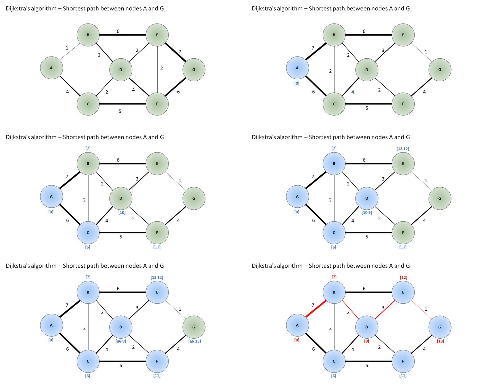
To see this process in action, the following video provides an excellent step-by-step walkthrough.

2. Implementation in Java

Let's translate this logic into a Java implementation. For this, we'll need:

• An adjacency list to represent the graph. A List<List<Node>> is a good choice, where Node is a simple class holding a destination vertex and an edge weight.
• A PriorityQueue to store pairs of (distance, vertex). We can use a custom class for this that implements Comparable, or, as is common in competitive programming, use a simple int[] array and provide a lambda expression for the comparator.
• A dist array to store the final shortest path distances.

Here is a full, runnable example. The structure should feel familiar after our work on Prim's algorithm.

import java.util.*;

public class DijkstrasAlgorithm {

    // Inner class to represent a node in the adjacency list (neighbor and edge weight)
    static class AdjNode {
        int vertex;
        int weight;

        AdjNode(int v, int w) {
            this.vertex = v;
            this.weight = w;
        }
    }

    // Inner class for the priority queue to store (vertex, distance) pairs
    static class PQNode implements Comparable<PQNode> {
        int vertex;
        int distance;

        PQNode(int v, int d) {
            this.vertex = v;
            this.distance = d;
        }

        @Override
        public int compareTo(PQNode other) {
            return Integer.compare(this.distance, other.distance);
        }
    }

    public static int[] dijkstra(int V, List<List<AdjNode>> adj, int source) {
        // Distance array, initialized to infinity
        int[] dist = new int[V];
        Arrays.fill(dist, Integer.MAX_VALUE);

        // Min-priority queue to select the node with the smallest distance
        PriorityQueue<PQNode> pq = new PriorityQueue<>();

        // Start with the source node
        dist[source] = 0;
        pq.add(new PQNode(source, 0));

        while (!pq.isEmpty()) {
            // Get the node with the smallest distance from the source
            PQNode current = pq.poll();
            int u = current.vertex;
            int d = current.distance;
            
            // This is an optimization. If we have already found a shorter path to u,
            // the entry in the PQ is outdated. We can ignore it.
            if (d > dist[u]) {
                continue;
            }

            // Explore neighbors of the current node
            for (AdjNode neighbor : adj.get(u)) {
                int v = neighbor.vertex;
                int weight = neighbor.weight;

                // Relaxation step
                if (dist[u] + weight < dist[v]) {
                    dist[v] = dist[u] + weight;
                    // Add the updated neighbor to the priority queue
                    pq.add(new PQNode(v, dist[v]));
                }
            }
        }

        return dist;
    }

    public static void main(String[] args) {
        int V = 9;
        int source = 0;

        List<List<AdjNode>> adj = new ArrayList<>();
        for (int i = 0; i < V; i++) {
            adj.add(new ArrayList<>());
        }

        // Example graph from FinalRoundAI article
        addEdge(adj, 0, 1, 4);
        addEdge(adj, 0, 7, 8);
        addEdge(adj, 1, 2, 8);
        addEdge(adj, 1, 7, 11);
        addEdge(adj, 2, 3, 7);
        addEdge(adj, 2, 5, 4);
        addEdge(adj, 2, 8, 2);
        addEdge(adj, 3, 4, 9);
        addEdge(adj, 3, 5, 14);
        addEdge(adj, 4, 5, 10);
        addEdge(adj, 5, 6, 2);
        addEdge(adj, 6, 7, 1);
        addEdge(adj, 6, 8, 6);
        addEdge(adj, 7, 8, 7);

        int[] shortestDistances = dijkstra(V, adj, source);

        System.out.println("Shortest distances from source vertex " + source + ":");
        for (int i = 0; i < V; i++) {
            System.out.println("Vertex " + i + ": " + (shortestDistances[i] == Integer.MAX_VALUE ? "Infinity" : shortestDistances[i]));
        }
    }

    // Helper to add edges for an undirected graph
    public static void addEdge(List<List<AdjNode>> adj, int u, int v, int weight) {
        adj.get(u).add(new AdjNode(v, weight));
        adj.get(v).add(new AdjNode(u, weight));
    }
}

For a more detailed breakdown of a similar implementation, you can refer to this article.

3. A Critical Limitation: Negative Edge Weights

Dijkstra's algorithm's greedy strategy fundamentally relies on one assumption: all edge weights are non-negative. When this is true, once we declare a vertex u as "visited," we can be certain we have found its shortest path. Any other path to u we discover later will have to go through more edges, and since edge weights aren't negative, the path can't possibly be shorter.

If a graph contains a negative edge, this assumption breaks. A path with more edges might actually have a lower total weight. If there's a negative-weight cycle, you could loop forever, making the path infinitely short.

4. Complexity Analysis

For interviews and competitive programming, knowing the complexity is non-negotiable.

• Time Complexity: The performance is determined by the priority queue operations.

  • We add each vertex to the visited set exactly once.
  • Each edge (u, v) is considered during the relaxation step when we process u. This can lead to at most E add operations on the priority queue.
  • We perform V poll operations to extract each vertex once.
  • Both add and poll on a binary heap (like Java's PriorityQueue) take $O(\log N)$ time, where $N$ is the number of elements in the queue. The queue size can go up to $V$.
  • Therefore, the total time complexity is $O(E\log V+V\log V)$. For a connected graph where $E\ge V-1$, this simplifies to $O(E\log V)$.

• Space Complexity:

  • Adjacency list: $O(V+E)$.
  • dist array: $O(V)$.
  • Priority Queue: In the worst case, can store an entry for each vertex, so $O(V)$.
  • The total space complexity is $O(V+E)$.

Conclusion

In this lesson, you've mastered Dijkstra's algorithm, a cornerstone of graph theory.

Key Takeaways:

• Dijkstra's algorithm finds the single-source shortest paths in a weighted graph.
• It is a greedy algorithm that always explores the unvisited node with the smallest cumulative distance from the source.
• A min-priority queue is essential for an efficient implementation, leading to a time complexity of $O(E\log V)$.
• A critical limitation: Dijkstra's algorithm only works for graphs with non-negative edge weights.

Preview of the Next Lesson:
We've just identified a key weakness in Dijkstra's algorithm. So, what do we do if our graph does have negative edge weights? In our next lesson, we will learn the Bellman-Ford algorithm. It is slower than Dijkstra's but is more robust, as it can handle negative edge weights and can even be used to detect the presence of negative-weight cycles.