Matrix Operations with NumPy

1. The Determinant: A Measure of Transformation Scaling

Let's start with the first question. When we apply a linear transformation (like the ones we saw last lesson) to a shape on a grid, the shape's area changes. The determinant is a single number that tells us the exact factor by which this scaling happens.

To see this in action, let's watch a short video that brilliantly visualizes the concept.

As the video illustrates, the determinant quantifies how much a transformation expands or contracts space.

Geometric Interpretation

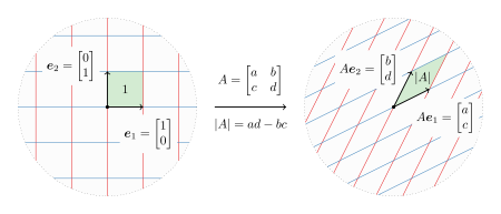
Let's formalize this. For a 2D transformation represented by a matrix $A$, the absolute value of its determinant, written as $|\det (A)|$, tells you how the area of any region changes.

• If $|\det (A)|>1$, the transformation expands the area.
• If $|\det (A)|<1$, the transformation contracts the area.
• If $|\det (A)|=1$, the transformation preserves the area (like a pure rotation).

The image below shows how the unit square, formed by basis vectors $\hat{i}$ and $\hat{j}$, is transformed into a parallelogram. The area of this new parallelogram is precisely $|\det (A)|$.

What if the determinant is zero or negative?

• Negative Determinant: A negative determinant means the orientation of space has been "flipped" or inverted. Imagine taking a piece of paper, flipping it over, and then stretching it. The flip corresponds to the negative sign. A reflection is a classic example of a transformation with a negative determinant.
• Zero Determinant: This is a critical case. If $\det (A)=0$, it means the transformation squishes space into a lower dimension. For example, a 2D plane is collapsed onto a single line or even a point. The resulting "area" is zero. This tells us something profound: the transformation has lost information and cannot be undone.

To solidify this, let's read a short text that summarizes these geometric ideas.

Calculating the Determinant with NumPy

While there are manual formulas for calculating determinants, they quickly become complex for matrices larger than 2x2. In practice, we'll always use a library like NumPy.

For a 2x2 matrix $A=\left[\begin{array}{cc}a& b\\ c& d\end{array}\right]$, the formula is simple: $\det (A)=ad-bc$.

For anything larger, we use numpy.linalg.det().

Let's see it in code.

import numpy as np

# A matrix that expands area
A = np.array([[3, 0],
              [0, 2]])
# This matrix scales x by 3 and y by 2. 
# A unit square (area 1) becomes a rectangle of 3x2 (area 6).
print(f"Matrix A:\n{A}")
print(f"Determinant of A: {np.linalg.det(A):.1f}")
print("-" * 20)

# A matrix that includes rotation and shear
B = np.array([[1, 2],
              [-1, 3]])
print(f"Matrix B:\n{B}")
print(f"Determinant of B: {np.linalg.det(B):.1f}")
print("-" * 20)

# A matrix that collapses space (a singular matrix)
# Notice that the second column is twice the first column.
C = np.array([[1, 2],
              [2, 4]])
print(f"Matrix C:\n{C}")
print(f"Determinant of C: {np.linalg.det(C):.1f}")

The output for matrix C will be 0.0, confirming our intuition that if the columns are linearly dependent (one is a multiple of the other), the transformation collapses space, resulting in zero area.

2. The Matrix Inverse: Undoing a Transformation

Now for our second question: can we reverse a transformation? If a matrix $A$ transforms a vector $x$ to a new position $y$ ($Ax=y$), is there a matrix that can take $y$ back to $x$?

Yes, and this is called the inverse matrix, denoted as $A^{-1}$.

The inverse matrix $A^{-1}$ is defined by the property:

Where $I$ is the identity matrix—a matrix with 1s on the diagonal and 0s elsewhere. The identity matrix is the "do nothing" transformation; multiplying any vector by $I$ leaves it unchanged.

Invertibility and the Determinant

Here is the crucial link: A square matrix $A$ has an inverse if and only if its determinant is non-zero.

Why?
As we saw, if $\det (A)=0$, the transformation squishes space into a lower dimension. This process is irreversible because information is lost. Multiple input vectors get mapped to the same output vector, so there's no unique way to go backward. A matrix with a zero determinant is called singular or non-invertible.

If $\det (A)\ne 0$, the transformation is one-to-one, no information is lost, and we can define a unique inverse transformation $A^{-1}$.

Let's read a concise explanation of this fundamental connection.

Finding the Inverse with NumPy

To compute the inverse of a matrix, we use numpy.linalg.inv().

Let's try this with the matrices from our previous example.

# Recall matrix B from before
B = np.array([[1, 2],
              [-1, 3]])
print(f"Matrix B:\n{B}")
print(f"Determinant of B: {np.linalg.det(B):.1f}\n") # Determinant is 5, so it's invertible

# Calculate the inverse
B_inv = np.linalg.inv(B)
print(f"Inverse of B:\n{B_inv}\n")

# Verify that B @ B_inv is the identity matrix
identity_check = B @ B_inv
print(f"B @ B_inv:\n{identity_check}")
# Note: due to floating point precision, you might see very small numbers
# like 1.11e-16 instead of exactly 0. np.allclose(identity_check, np.identity(2)) is a good way to check.
print("-" * 20)

# Now, let's try to invert the singular matrix C
C = np.array([[1, 2],
              [2, 4]])
print(f"Matrix C:\n{C}")
print(f"Determinant of C: {np.linalg.det(C):.1f}")

try:
    C_inv = np.linalg.inv(C)
except np.linalg.LinAlgError as e:
    print(f"\nCould not invert matrix C. Error: {e}")

As expected, NumPy raises a LinAlgError when we attempt to invert C because it is a singular matrix (its determinant is zero).

A final practical note: While the inverse is a powerful theoretical tool, directly computing it can sometimes be numerically unstable if the determinant is very close to zero. In many ML applications, to solve a system like $Ax=b$, we prefer using dedicated solvers (like np.linalg.solve(A, b)) over computing the inverse and multiplying ($x=A^{-1}b$).

Conclusion

Great job today! We've connected the abstract ideas of determinants and inverses to the visual, geometric behavior of matrices we explored in the last lesson.

Key Takeaways:

• The determinant of a matrix is a scalar value that represents the factor by which a linear transformation scales area (in 2D) or volume (in 3D).
• A zero determinant signifies that the transformation collapses space into a lower dimension, and the matrix is singular (non-invertible).
• A negative determinant indicates that the transformation also flips the orientation of space.
• The inverse matrix, $A^{-1}$, "undoes" the transformation of $A$. It exists if and only if $\det (A)\ne 0$.
• In NumPy, we use np.linalg.det() to compute the determinant and np.linalg.inv() to find the inverse.

Preview of the Next Lesson:

We've seen how matrices transform the entire space. But are there any vectors that are special? For instance, are there vectors that don't change their direction during a transformation, only their length? The answer is yes. These special vectors are called eigenvectors, and we will explore them in our next lesson. They reveal the fundamental axes of a transformation and are one of the most important concepts in linear algebra, with direct applications in machine learning algorithms like Principal Component Analysis (PCA).