Hello! Welcome back to our introduction to machine learning.
In our last lesson, we established the three main paradigms of machine learning: supervised, unsupervised, and reinforcement learning. We focused on supervised learning, where models learn from labeled data to make predictions. This raised a crucial question: how do we know if a model has truly learned a pattern, or if it has just memorized the training data? A model that seems perfect on the data it was trained on can often fail spectacularly when faced with new, unseen data.
Today, we'll tackle this problem head-on. Our goal is to explain the bias-variance tradeoff, one of the most fundamental concepts in machine learning. Understanding this tradeoff is the key to diagnosing why a model is performing poorly and choosing the right strategy to improve it. It's the difference between blindly adjusting parameters and making informed decisions to build robust, effective models.
1. Building an Intuition for Bias and Variance
Before we dive into the technical details, let's build some intuition with an analogy and a visual.
The Bias-Variance Tradeoff: Why Your Models Fail (And How to Fix Them)
This article from Let's Data Science provides a fantastic analogy to understand bias and variance. It compares them to two different types of students preparing for an exam.
Read the introductory section and the part titled "The Analogy: Studying for an Exam". Think about why both the "Slacker" and the "Memorizer" would perform poorly on a fair exam.
As the analogy illustrates:
- High Bias is like the "Slacker" student. The model is too simple and makes overly strong assumptions, failing to capture the underlying patterns in the data. This is called underfitting.
- High Variance is like the "Memorizer" student. The model is too complex and fits the training data too closely, including the noise. It's not flexible enough to generalize to new, slightly different data. This is called overfitting.
Another popular way to visualize bias and variance is with a target. Imagine the bullseye is the true value we want to predict. Each shot is a prediction from a model trained on a different subset of our data.

Here's how to interpret the target:
- Low Bias, Low Variance (Top-Left): The ideal scenario. Predictions are accurate and consistent.
- High Bias, Low Variance (Top-Right): The model is consistent but consistently wrong. It's underfitting.
- Low Bias, High Variance (Bottom-Left): The predictions are, on average, correct, but they are scattered. The model is sensitive to the specific training data. It's overfitting.
- High Bias, High Variance (Bottom-Right): The worst case. Predictions are inaccurate and inconsistent.
2. The Tradeoff and Model Complexity
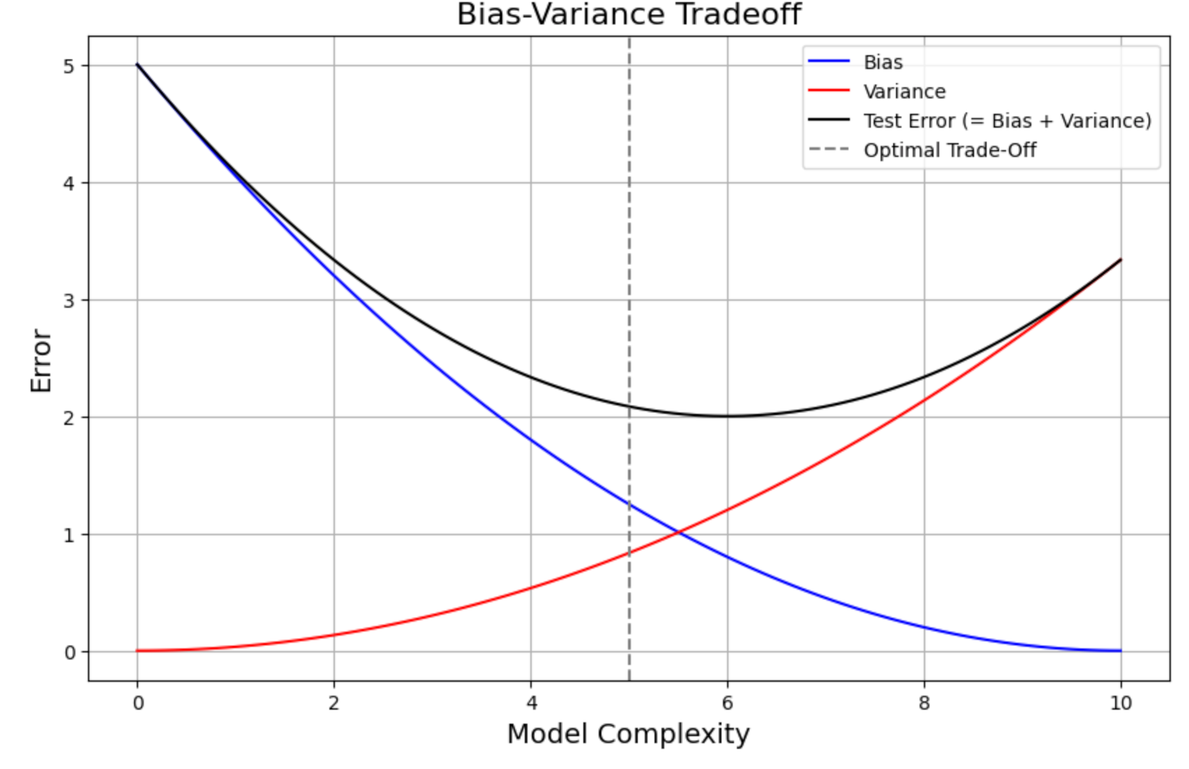
Bias and variance are often in tension with each other. A simple model (like a straight line for non-linear data) has high bias and low variance. A very complex model (like a high-degree polynomial that wiggles to hit every data point) has low bias but high variance. The challenge is finding the right level of model complexity that balances the two.
Let's watch a video from Stanford University that explains this relationship and introduces the mathematical decomposition of error.
Statistical Learning: 2.3 Model Selection and Bias Variance Tradeoff
This lecture segment from Stanford Online, presented by one of the authors of the seminal textbook 'An Introduction to Statistical Learning', formally breaks down model error and visualizes the tradeoff.
Watch the segment from 01:57 to 08:34. As you watch, focus on: The U-shaped curve (01:57 - 05:49): Notice how the training error (gray line) always decreases as the model gets more complex, but the test error (red line) decreases and then increases. The decomposition of error (05:49 - 08:34): Pay close attention to how the total expected error is broken down into three components: Bias, Variance, and Irreducible Error.
As the video explained, the total error of a model can be broken down into three parts.
3. The Mathematical View of Error
Let's formalize the decomposition you saw in the video. For a supervised learning model, the expected error for a new, unseen data point can be expressed as:
Let's break this down:
- Irreducible Error (): This is the inherent noise or randomness in the data itself. No model, no matter how perfect, can eliminate this error. It represents the lower bound on the error that any model can achieve.
- Bias: This term measures the difference between the average prediction of our model (if we were to train it on many different datasets) and the true underlying relationship. High bias means our model's fundamental assumptions are wrong (e.g., assuming a linear relationship when it's curved).
- Variance: This term measures how much the predictions of our model would change if we used a different training dataset. High variance means our model is unstable and highly dependent on the specific data points it was trained on—it's learning the noise.
The "tradeoff" means that as we decrease bias (by making our model more complex), we typically increase variance, and vice-versa. Our goal is not to eliminate bias or variance entirely, but to find a model complexity that minimizes their sum.
Test your understanding!
A data scientist trains a decision tree model to predict house prices.
- Scenario A: They limit the tree to a maximum depth of 2 (very simple).
- Scenario B: They let the tree grow to a maximum depth of 30 (very complex), fitting the training data almost perfectly.
Which scenario is likely to have high bias, and which is likely to have high variance? Explain why.
Show answer
- Scenario A (depth=2) is likely to have high bias. The model is too simple to capture the complex relationships between a house's features and its price. It will underfit the data, leading to poor predictions on both the training and test sets.
- Scenario B (depth=30) is likely to have high variance. The model is so complex that it has likely memorized the specific training data, including its random noise. While it will have very low error on the training set, it will fail to generalize to new data and will have a high error on the test set. It is overfitting.
4. How to Diagnose and Fix Bias and Variance Issues
In the real world, we can't directly calculate bias and variance because we don't know the "true" function. However, we can diagnose whether our model is suffering from high bias or high variance by comparing its performance on the training data versus a separate test (or validation) set.
The same article we started with provides a practical guide for this.
The Bias-Variance Tradeoff: Why Your Models Fail (And How to Fix Them)
Now let's learn how to spot these problems and what to do about them. This part of the article provides a clear summary of symptoms and solutions.
Read the sections "How do we detect Bias and Variance?" and "Practical Guide: Fixing Your Model". Focus on the table that maps symptoms to a diagnosis and the bulleted lists of fixes for both underfitting and overfitting.
Here is a summary of the diagnostic "cheat sheet":
| Symptom | Diagnosis | Primary Problem |
|---|---|---|
| High Training Error & High Test Error | High Bias | Underfitting |
| Low Training Error & High Test Error | High Variance | Overfitting |
And here are the common remedies:
To Fix High Bias (Underfitting):
- Increase Model Complexity: Switch to a more powerful model (e.g., from linear regression to a random forest).
- Add More Features (Feature Engineering): Provide the model with more information.
- Decrease Regularization: Reduce constraints that might be making the model too simple.
To Fix High Variance (Overfitting):
- Get More Training Data: This is often the most effective solution. More data helps the model learn the true signal instead of the noise.
- Reduce Model Complexity: Use a simpler model or reduce the complexity of the current one (e.g., prune a decision tree).
- Add Regularization: Introduce a penalty for complexity, which forces the model to be simpler.
Conclusion
Today, we've explored the central challenge in supervised learning: balancing bias and variance. This isn't just a theoretical concept; it's a practical framework you will use constantly to build better models.
Key Takeaways:
- Total Error in a model is a sum of Bias², Variance, and Irreducible Error.
- Bias is error from wrong assumptions, leading to underfitting. A high-bias model is too simple and performs poorly on both training and test data.
- Variance is error from sensitivity to the training data, leading to overfitting. A high-variance model is too complex, performs perfectly on training data, but fails on new data.
- The Bias-Variance Tradeoff is the tension between these two errors. Increasing model complexity typically decreases bias but increases variance.
- We can diagnose these issues by comparing training error and test error and apply specific strategies to fix them.
Preview of the Next Lesson:
We've repeatedly mentioned the importance of "training data" and "test data" for diagnosing bias and variance. But how do we do this properly? If we use our test data to tune our model, we risk having it "leak" information, giving us an overly optimistic view of our model's performance. In the next lesson, we will learn how to properly split data into training, validation, and test sets to build and evaluate models in a robust and reliable way.