Derivatives of Single-Variable Functions

1. The "Why": What is a Derivative?

Before we start calculating, let's build an intuition for what a derivative is and why it's so fundamental to machine learning.

The Core Idea: Instantaneous Rate of Change

Imagine your machine learning model has a single parameter (let's call it $x$) and a loss function $L(x)$ that measures how poorly the model is performing. To improve the model, you need to adjust $x$. But in which direction should you adjust it, and by how much? You want to move in the direction where the loss decreases most rapidly.

The derivative gives us this information. It tells us the instantaneous rate of change of a function at a specific point. Geometrically, this is the slope of the line tangent to the function's curve at that point.

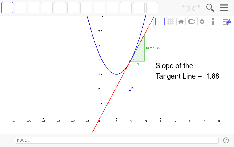
To understand this better, let's watch a short video that introduces the derivative as the slope of a tangent line on a curve.

The Formal Definition: The Limit

So, how do we calculate this "slope at a single point"? We can approximate it by taking two points on the curve that are very, very close together and calculating the slope of the line connecting them (a secant line). The derivative is what we get when we take the limit of this slope as the distance between the two points approaches zero.

This gives us the formal definition of the derivative of a function $f(x)$, denoted as $f^{\prime }(x)$ or $\frac{df}{dx}$:

$f^{\prime }(x)={\lim }_{h\to 0}\frac{f(x+h)-f(x)}{h}$

Let's break this down:

• $h$ is a very small change in the input $x$.
• $f(x+h)-f(x)$ is the resulting change in the function's output (the "rise").
• The denominator, $h$, is the change in the input (the "run").
• The ${\lim }_{h\to 0}$ part means we are looking at what happens to this ratio as the change $h$ becomes infinitesimally small.

The following video provides a clear explanation of this formula and its components.

Given your background in computer science, you might appreciate a computational perspective on this. The text below demonstrates this limit process with Python code, showing how the calculated ratio gets closer and closer to the true derivative as the step size (epsilon, or our $h$) gets smaller.

2. The "How": Rules for Differentiation

Using the limit definition every time is time-consuming. Fortunately, mathematicians have developed a set of rules that make finding derivatives much faster. For today's lesson, we'll focus on the rules needed to differentiate any polynomial function.

These are the essential rules:

1. The Constant Rule: The derivative of a constant is zero.

   • If $f(x)=c$, then $f^{\prime }(x)=0$.
   • This makes sense: a constant function is a horizontal line, and its slope is always zero.

2. The Power Rule: To find the derivative of $x^n$, you bring the exponent down as a multiplier and then subtract one from the exponent.

   • If $f(x)=x^n$, then $f^{\prime }(x)=n\cdot x^{n-1}$.
   • This is the most important rule for polynomials. For example, the derivative of $x^3$ is $3x^2$.

3. The Constant Multiple Rule: The derivative of a constant multiplied by a function is the constant times the derivative of the function.

   • If $f(x)=c\cdot g(x)$, then $f^{\prime }(x)=c\cdot g^{\prime }(x)$.
   • Example: The derivative of $5x^3$ is $5\cdot (3x^2)=15x^2$.

4. The Sum/Difference Rule: The derivative of a sum (or difference) of functions is the sum (or difference) of their derivatives.

   • If $f(x)=g(x)+h(x)$, then $f^{\prime }(x)=g^{\prime }(x)+h^{\prime }(x)$.
   • This allows us to differentiate a polynomial term by term.

Let's watch a video that demonstrates these rules with clear examples.

3. Extending the Power Rule

The power rule is even more versatile than it first appears. It also works for negative and fractional exponents, which allows us to easily differentiate rational functions (like $\frac{1}{x^2}$) and radical functions (like $\sqrt{x}$).

The key is to first rewrite the function in the form $x^n$:

• $\frac{1}{x^2}$ can be rewritten as $x^{-2}$.
• $\sqrt{x}$ can be rewritten as $x^{1/2}$.

Once rewritten, you can apply the power rule just as before. Let's see this in action.

4. Practical Application: Derivatives in Python

While manual calculation is crucial for understanding, in practice you'll use libraries to compute derivatives. For symbolic computation (manipulating mathematical expressions directly), Python's sympy library is the perfect tool.

The image below shows how to use sympy to define a function and find its derivative automatically.

This workflow is incredibly powerful. You can define complex functions and get their exact derivatives without manual calculation, which is essential as we move towards more complex models in machine learning.

Conclusion

In this lesson, we laid the foundational groundwork for calculus in machine learning. You've learned not just how to compute derivatives, but also what they represent.

Key Takeaways:

• A derivative measures the instantaneous rate of change of a function, which is geometrically represented as the slope of the tangent line.
• The formal limit definition, ${\lim }_{h\to 0}\frac{f(x+h)-f(x)}{h}$, is the principle from which all differentiation is derived.
• We can efficiently compute derivatives using a set of rules, most notably the power rule, constant multiple rule, and sum rule.
• The power rule applies to integer, negative, and fractional exponents, making it widely applicable.
• In Python, the sympy library is the standard tool for performing symbolic differentiation.

Preview of the Next Lesson:

We've now mastered finding the derivative of functions with a single input variable, like $f(x)$. However, a real machine learning loss function depends on many parameters (weights and biases), making it a function of thousands or even millions of variables. How do we find the "slope" in such a high-dimensional space?

To answer this, we need to extend our concept of the derivative. In the next lesson, we will learn how to calculate partial derivatives of multivariable functions, which allows us to see how the function changes when we alter just one variable at a time.