Gradient Descent: Iteration and Learning Rate

Hello! Welcome back to our calculus module.

In our last lesson, we assembled the final piece of our mathematical toolkit: the Jacobian matrix. We learned how to compute the gradient for functions with multiple inputs and outputs, and we saw how the vector chain rule provides an elegant way to find derivatives of complex, nested functions—like those in a neural network. We ended with a preview of how we could use these gradients to 'walk' down a function's surface to find its lowest point.

Today, we will dive deep into that very idea. This lesson introduces Gradient Descent, arguably the most important optimization algorithm in machine learning. It's the engine that drives model training, from simple linear regression to the most complex deep neural networks.

Our goal is to understand the iterative process of gradient descent and explain the crucial role of the learning rate. By the end of this lesson, you'll have a strong conceptual grasp of how a machine learning model actually learns.

1. The Goal: Finding the Bottom of the Hill

Before we get into the mechanics, let's establish the "why". In machine learning, we train a model by defining a cost function (also called a loss function). This function takes the model's parameters (e.g., weights and biases) as input and outputs a single number that measures how "wrong" the model's predictions are compared to the actual data. A high cost means the model is performing poorly; a low cost means it's doing well.

The goal of training is to find the set of parameters that results in the minimum possible cost. Gradient descent is the algorithm we use to find this minimum.

The following video provides a brilliant conceptual overview, framing this optimization problem as finding the lowest point in a vast, multidimensional landscape.

Gradient descent, how neural networks learn | Deep Learning Chapter 2

This video from 3Blue1Brown will help you build a strong intuition for what we're trying to achieve. It visualizes the cost function as a surface and gradient descent as the process of walking downhill.

Watch the video from the beginning to 09:15. Focus on these key ideas: What a cost function represents. The analogy of finding a minimum by taking steps in the downhill direction. How the negative gradient provides this direction of steepest descent.

As the video explained, the gradient of the cost function, $\nabla C$ , points in the direction of the steepest ascent (the "uphill" direction). Therefore, to find the minimum, we want to move in the direction of the negative gradient, $- \nabla C$ . This is the core principle of gradient descent.

Gradient Descent Visualization — This image illustrates the iterative process. Starting from an initial position, gradient descent takes successive steps in the direction of the negative gradient, moving 'downhill' on the function's curve until it settles in a minimum.

2. The Gradient Descent Algorithm: Step-by-Step

Now that we have the intuition, let's formalize this "walking downhill" process into a concrete algorithm. Gradient descent is an iterative process, meaning it repeats a series of steps until it reaches a solution.

The process is as follows:

Initialize Parameters: Start by assigning random initial values to your model's parameters (e.g., weights w and bias b). This is your starting point on the cost function's landscape.
Compute the Gradient: Calculate the gradient of the cost function with respect to each parameter at the current parameter values. This tells you the direction of steepest ascent for each parameter.
Update Parameters: Adjust each parameter by taking a small step in the opposite direction of its gradient.
Repeat: Go back to step 2 and repeat the process. With each iteration, you should move closer to a minimum of the cost function.

The following video from StatQuest provides a fantastic, step-by-step walkthrough of this exact process using a simple linear regression example.

Gradient Descent, Step-by-Step

Watch this video to see the gradient descent algorithm in action. It starts by optimizing just one parameter (the intercept) to make the steps clear, before expanding to multiple parameters.

Watch the segments from 02:09-05:38, 07:18-10:43, 10:43-13:30, and the summary from 14:39-15:49. Pay close attention to: How the derivative (the slope of the cost curve) is used. How the step size is calculated. How the parameter is updated in each iteration. The final summary of the five key steps of the algorithm.

To summarize the video and formalize the update step, we can write it as a mathematical formula. For a parameter $θ$ (which could be a weight or a bias), the update rule in each iteration is:

θ_{new} = θ_{old} - α \cdot \frac{\partial C}{\partial θ}

Where:

$θ_{new}$ is the updated value of the parameter.
$θ_{old}$ is its current value.
$\frac{\partial C}{\partial θ}$ is the partial derivative of the cost function $C$ with respect to $θ$ (one component of the gradient).
$α$ (alpha) is the learning rate.

This brings us to the second part of our learning goal: understanding the crucial role of $α$ .

3. The Learning Rate: Choosing Your Step Size

The learning rate is a hyperparameter—a setting you choose before training begins—that controls how big of a step you take during each update. It scales the gradient, so a larger learning rate means a larger step.

Choosing the right learning rate is critical for gradient descent to work effectively.

If the learning rate is too small, the algorithm will take tiny steps. It will eventually reach the minimum, but it will take a very long time and many iterations, making the training process inefficient.
If the learning rate is too large, the algorithm will take huge steps. This can cause it to "overshoot" the minimum and bounce around wildly. In the worst case, the steps are so large that the cost actually increases with each iteration, and the algorithm diverges instead of converging.

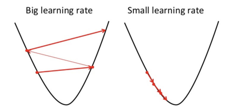
Impact of Learning Rate in Gradient Descent — This image perfectly visualizes the effect of the learning rate. A small learning rate leads to a slow but steady convergence. A large learning rate overshoots the minimum, oscillating back and forth and failing to find the optimal solution efficiently.

The key is to find a "Goldilocks" value—not too big, not too small—that allows for efficient convergence without overshooting. This is often done through experimentation.

To read a bit more about this process and see the update rule presented in another way, you can review the following short article.

Gradient Descent Optimization: A Simple Guide for Beginners

This article from Udacity, 'Gradient Descent Optimization', provides a concise summary of the algorithm's steps and key terms, including a clear definition of the learning rate.

Read the section 'How Gradient Descent Works'. It gives a clear, 5-step breakdown of the process and reinforces the definitions of Cost Function, Gradients, and Learning Rate.

Test your understanding!

You are training a machine learning model using gradient descent. After a few iterations, you plot the cost function's value and notice that it is steadily increasing instead of decreasing.

What is the most likely cause of this problem, and what is the first, most straightforward action you should take to fix it?

Show answer

The most likely cause is that the learning rate is too large. This is causing the algorithm to overshoot the minimum so dramatically that it ends up at a point with a higher cost after each step (divergence).

The first action to take is to reduce the learning rate. A common strategy is to try decreasing it by a factor of 10 (e.g., from 0.1 to 0.01) and run the training again to see if the cost starts to decrease.

Conclusion

In this lesson, we demystified the core process of how machine learning models learn. We've seen that it's not magic, but a methodical, iterative optimization process grounded in calculus.

Key Takeaways:

Gradient Descent is an iterative algorithm used to find the minimum of a cost function by adjusting a model's parameters.
The core idea is to repeatedly take steps in the direction of the negative gradient (the direction of steepest descent).
The iterative process involves: initializing parameters, computing the gradient of the cost, and updating the parameters using the update rule: $θ_{new} = θ_{old} - α \cdot \nabla C$ .
The learning rate ( $α$ ) is a critical hyperparameter that controls the step size. It must be carefully chosen to ensure efficient convergence without overshooting the minimum.

Preview of the Next Lesson:
We've covered the theory and the "why." Now it's time to put it into practice. In the next lesson, we will implement a basic gradient descent algorithm in Python. You'll write the code to perform these update steps and watch as your simple model learns to fit a line to data, right before your eyes

Recommended resources

1. The Goal: Finding the Bottom of the Hill

2. The Gradient Descent Algorithm: Step-by-Step

3. The Learning Rate: Choosing Your Step Size

Conclusion